Research Article: 2017 Vol: 18 Issue: 3
A Model To Explain The Monetary Trilemma Using Tools From Principles of Macroeconomics
Keywords
A2 Economic Education, The Teaching of Economics.
Introduction
The Economist Magazine (2016) labeled the monetary trilemma as one of six big ideas that explains how the world works. Feenstra and Taylor (2014 p. 457) state that the monetary trilemma “is one of the most important ideas in international macroeconomics.” The monetary trilemma or impossible trinity as economists sometimes call it, states that policy makers cannot simultaneously achieve exchange rate stability, pursue an independent monetary policy and allow free capital flows with other economies. Mundell (1961, 1962, 1963; Fleming 1962; McKinnon 1963) wrote path-breaking articles related to the issue of the trilemma. Obstfeld and Taylor (2017) examine the history of how governments have dealt with the monetary trilemma and relate their discussion to the desire by governments to maintain domestic financial stability, pursue autonomous financial policies and integrate domestic financial markets with global financial markets.
Figure 1 illustrates the monetary trilemma. The vertices represent desired goals of a monetary system. Any two vertices and the line between them represent the mix of open-economy results from attempting to achieve the two desired goals. Also, Krugman, Obstfeld and Melitz (2015, p. 547-548) for an explanation of a diagram similar to Figure 1 in the present paper.
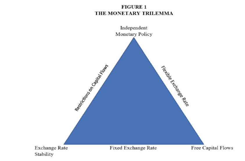
Figure 1: The Monetary Trilemma
Textbooks
Most undergraduate textbooks in International Economics do not discuss the monetary trilemma, perhaps because the authors believe the concept is too difficult for undergraduate students. The undergraduate International Economics textbooks that do explain the trilemma use models that go beyond the tools covered in courses in Principles of Macroeconomics. Feenstra and Taylor use the IS-LM-FX model to explain the monetary trilemma. Equilibrium in the goods market (IS) and equilibrium in the asset market (LM) are described as functions of the interest rate and income. Equilibrium in the foreign exchange market (FX) takes place where the domestic interest rate equals the world interest rate. Salvatore (2016) uses a comparable model to Feenstra and Taylor, the IS-LM-BP model, to explain the trilemma. The IS and LM curves are defined the same way as in Feenstra and Taylor and the BP line shows combinations of interest rate and income where there is neither a deficit nor surplus in the economy’s balance of payments. Krugman, Obstfeld and Melitz (2015) develop the DD-AA model in which they examine equilibrium in the goods market (DD) and equilibrium in the asset market (AA) as functions of the exchange rate and income to explain the trilemma. Van Marrewijk (2012) uses a model relating an economy’s current account to the economy’s real exchange rate to examine the trilemma. Sawyer and Sprinkle (2015) discuss the trilemma in the context of currency unions. Carbaugh (2015) introduces the monetary trilemma without having a formal model to explain it.
Textbooks in International Economics that do not explicitly discuss the monetary trilemma include Appleyard and Field (2010), Daniels and Van Hoose (2014), Gerber (2018), Husted and Melvin (2013), Kreinin and Clark (2013), Pugel (2016), Suranovic (2013), Thompson (2011), and Yarbrough and Yarbrough (2006).
Some textbooks in Intermediate Macroeconomics examine the monetary trilemma as part of their analysis of open economy monetary and fiscal policies. Mankiw (2016) does so using an IS-LM model with the exchange rate and income on the axes. Other textbooks in Intermediate Macroeconomics that cover the trilemma includes Dornbusch, Fischer and Startz (2014), Hubbard, O’Brien and Rafferty (2014), Jones (2018) and Mishkin (2012).
The purpose of the present paper is to illustrate the monetary trilemma in a model that uses tools developed in Principles of Macroeconomics.
The Model
The model in the present paper considers the market for products (goods and services), the money market and the foreign exchange market, which is broken down into the financial account and the current account. Figure 2 below illustrates the model.
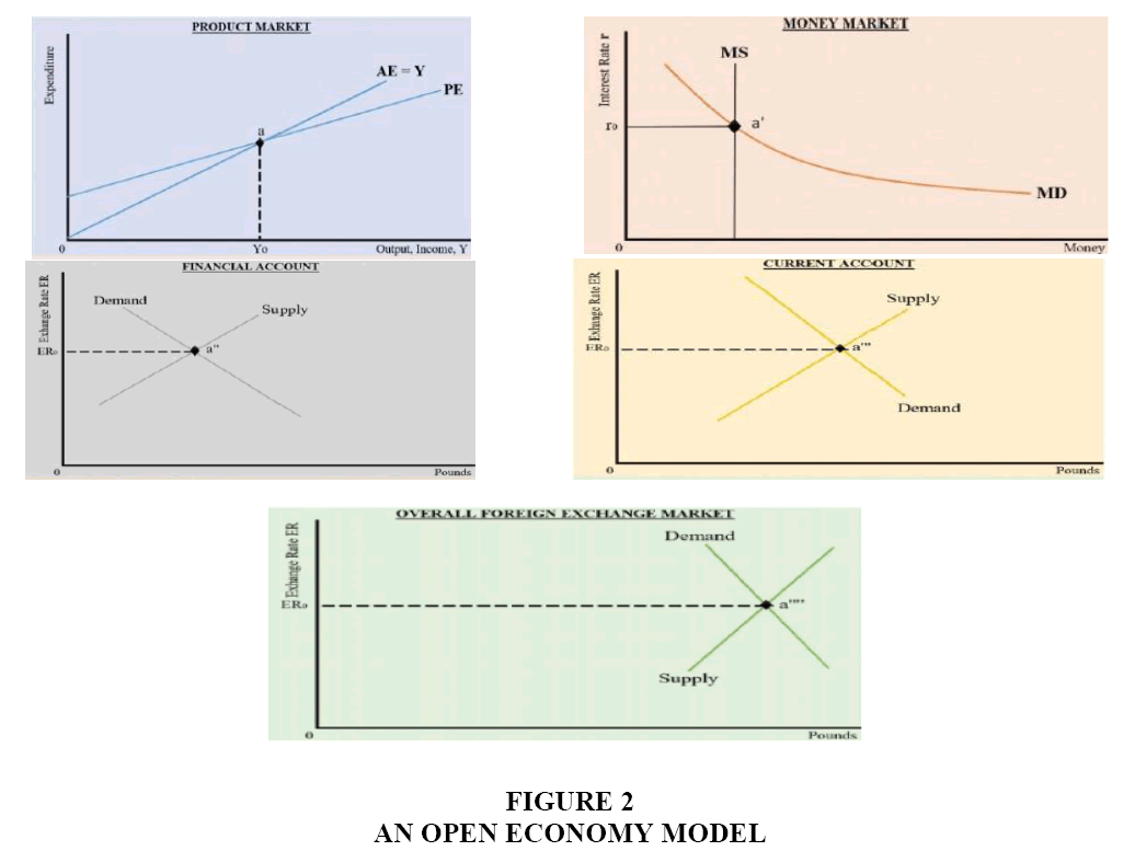
Figure 2: An Open Economy Model
The market for products assumes a fixed price level. Output of goods and services (Y) equals expenditure on goods and services, which is consumption (C) plus investment (I) plus government purchases (G) plus exports (EX) minus imports (IM). Consumption is positively related to disposable income (Y–Taxes); investment is negatively related to the interest rate (r); exports are negatively related to the exchange rate (ER); and imports are positively related to the exchange rate and positively related to disposable income. Since the price level is fixed, the nominal exchange rate, ER, is also the real exchange rate. The government levies lump sum levies Taxes (T).
The Keynesian Cross depicts the product market. The horizontal axis measures output (income) and the vertical axis measures expenditure. The 45 degree line reflects the identity between actual expenditure (AE) and output. Actual expenditure includes unplanned changes in inventories. Planned expenditure (PE)=C+IP+G+EX–IM, where IP=Planned investment. PE is a positively sloped line, as the marginal propensity to consume (change in consumption/change in disposable income) is greater than the marginal propensity to import (change in imports/change in disposable income), with both values being greater than zero and less than one. The slope of the PE line equals the marginal propensity to consume minus the marginal propensity to import.
The central bank sets the money supply (MS), which is independent of the interest rate. The demand for money (MD) specifies that the quantity demanded for money is a negative function of the interest rate and a positive function of income. Money is measured on the horizontal axis and the interest rate is measured on the vertical axis.
The financial account is shown with pounds (the domestic currency) measured on the horizontal axis and the exchange rate (dollar price per pound) measured on the vertical axis. The quantity demanded for pounds, which reflects the purchase of domestic assets by foreign investors, is negatively related to the exchange rate. The quantity supplied of pounds, which reflects the purchase of foreign assets by domestic investors, is positively related to the exchange rate.
Financial (capital) inflows are positively related to the domestic interest rate and financial (capital) outflows are negatively related to the domestic interest rate. Hence, an increase in the domestic interest rate shifts the demand for pounds to the right and shifts the supply of pounds to the left. A decrease in the domestic interest rate shifts the demand for pounds to the left and shifts the supply of pounds to the right.
The model could assume that the domestic interest rate is tied directly to the world interest rate, so that the two interest rates are equal. Alternatively, the model could assume that domestic securities are imperfect substitutes for world securities and/or that investors are concerned that the domestic exchange rate may change unexpectedly; in this case, the domestic interest rate need not equal the world interest rate. To illustrate the monetary trilemma, the results are the same regardless of which assumption is made on the domestic interest rate versus the world interest rate. It is more general to assume that the domestic interest rate need not equal the world interest rate and that assumption is made here.
In the current account, the quantity demanded for pounds, which reflects payments by foreign buyers for the economy’s exports of goods and services, is negatively related to the exchange rate. The quantity supplied of pounds, which reflects the economy’s payment for imports of goods and services, is positively related to the exchange rate. As imports are positively related to disposable income, an increase in disposable income shifts the supply of pounds to the right and a decrease in disposable income shifts the supply of pounds to the left.
For ease of exposition, it is assumed initially that the exchange rate is such that the financial account and current account are both zero. Point a shows equilibrium in the product market; point a' shows equilibrium in the money market; point a'' shows the financial account to be zero; and point a''' shows the current account to be zero. In the overall foreign exchange market, which is the combined financial and current accounts, equilibrium is at point a''''.
Exchange Rate Stability and Free Capital Flows Lead to a Loss of An Independent Monetary Policy
Let the central bank increase the money supply, which lowers the interest rate. Planned investment rises, which raises planned expenditure and income. The increase in income raises money demand, causing the interest rate to rise somewhat, which causes planned investment and planned expenditure to decline somewhat. As income rises, consumption and imports rise along a given PE line.
The drop in the interest rate leads to a net capital outflow, which increases the supply of pounds and reduces the demand for pounds in the financial account. At the original exchange rate, there is an excess quantity supplied of pounds in the foreign exchange market representing financial account transactions.
The higher income raises imports and increases the supply of pounds on the foreign exchange market representing current account transactions. At the original exchange rate, there is an excess quantity supplied of pounds representing current account transactions. In the overall foreign exchange market, there is an excess quantity supplied of pounds at the original exchange rate.
Figure 3 below summarizes the net results of the analysis above. The money supply increases to MS1 and money demand increases to MD1. The interest rate falls to r1, which causes planned investment to rise. Planned expenditure rises to PE1 and income rises to Y1. Consumption rises by the marginal propensity to consume times (Y1–Y0); imports rise by the marginal propensity to import times (Y1 –Y0). At exchange rate ER0, there is an excess quantity supplied of bc pounds reflecting financial market transactions, an excess quantity supplied of de pounds reflecting current account transactions and an excess quantity supplied of fg pounds in the overall foreign exchange market, where fg=bc+de.
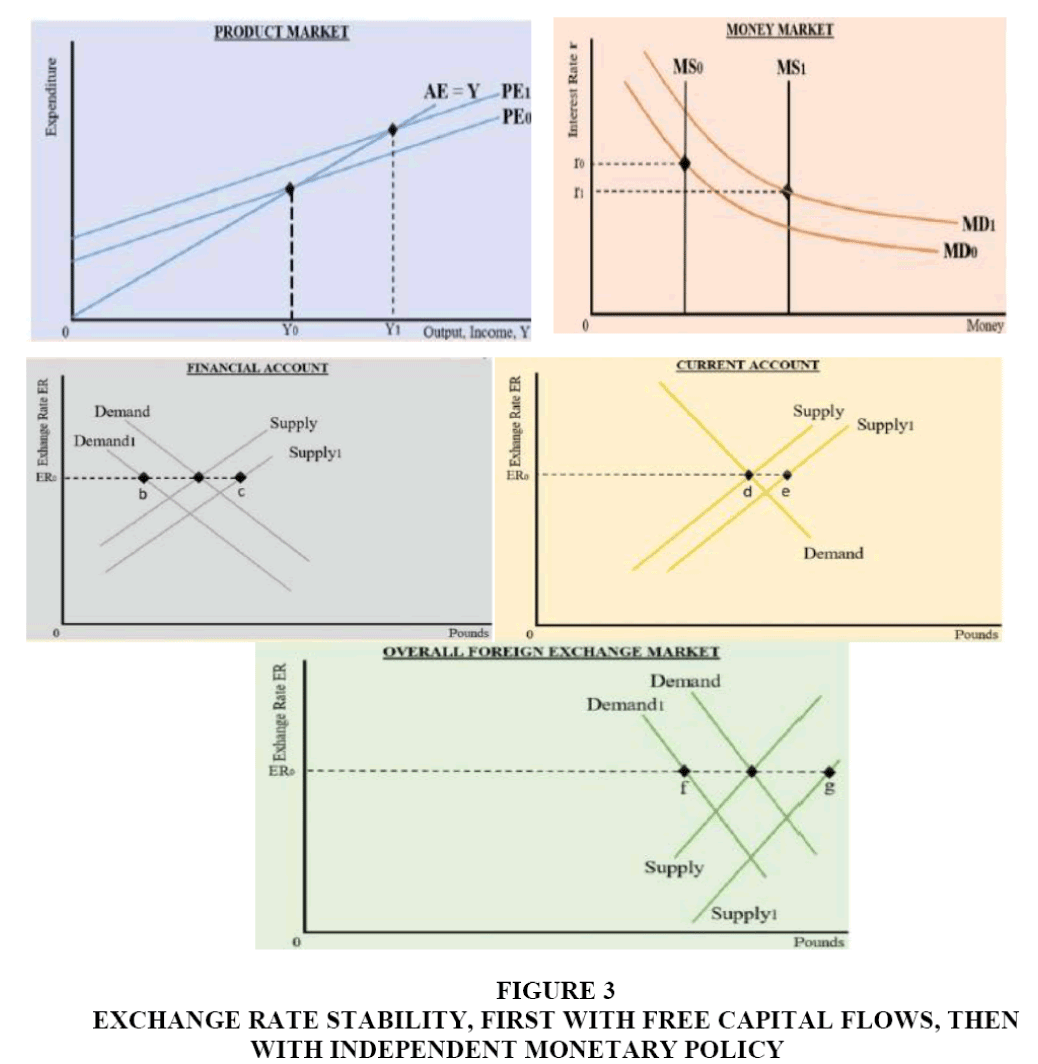
Figure 3: Exchange Rate Stability, First with Free Capital Flows, Then with Independent Monetary Policy
If policy makers wish to keep the exchange rate fixed at ER0 and allow unfettered capital flows across the economy’s borders, then the central bank sells foreign reserves and buys the excess quantity supplied of pounds on the foreign exchange market. The central bank activity reduces the money supply. To reach equality between the quantity demanded for and quantity supplied of pounds in the overall foreign exchange market, the interest rate rises to its original level (r0) and income returns to its original level (Y0); otherwise, the excess quantity supplied of pounds persists in the overall foreign exchange market. Accordingly, the economy returns to PE0; the money supply returns to MS0; and money demand returns to MD0. The financial and current accounts return to zero and the quantity demanded equals the quantity supplied of pounds at exchange rate ER0 in the overall foreign exchange market.
One change occurs in the central bank’s balance sheet. When the central bank increased the money supply, it bought government bonds in the open market. When it intervened on the foreign exchange market, it sold foreign reserves (dollars) and bought pounds. Hence, on its balance sheet (not provided in the paper), the increase in the value of government bonds is just offset by the loss in the value of foreign reserves, both measured in pounds.
The increase in the money supply (MS1–MS0) in Figure 3 equaled the value of the government bonds purchased by the central bank times by the economy’s money multiplier (whatever it happens to be). Then the money supply returned to its original level (MS0), since the drop in the money supply equaled the reduction of the central bank’s holdings of foreign reserves times the money multiplier.
If policy makers wish to maintain exchange rate stability and allow free cross-border capital flows, they lose the ability to pursue an independent monetary policy.
Exchange Rate Stability and an Independent Monetary Policy Require Restrictions on Capital Flows
Figure 3 can be used also to illustrate the need for financial account restrictions if policy makers wish to pursue monetary policy yet keep the exchange rate fixed. Given the initial increase in money supply to MS1 in Figure 3, at the initial exchange rate ER0 there is an excess quantity supplied of fg pounds in the overall foreign exchange market. If all current account transactions are to proceed and the monetary expansion is not to be reversed, then capital flows must be restricted to lead to a balance between the quantity supplied of and quantity demanded for pounds in the overall foreign exchange market at exchange rate ER0. Since there is an excess quantity supplied of pounds on the overall foreign exchange market, policy makers presumably would place restrictions on converting pounds to foreign currency (dollars in this case) on financial account transactions.
An independent monetary policy and exchange rate stability are incompatible with free cross-border capital flows.
An Independent Monetary Policy and Free Capital Flows Lead to a Loss of Exchange Rate Stability
Let policy makers wish to pursue an independent monetary policy and allow capital to flow freely across its country’s borders. An increase in the money supply lowers the interest rate, which raises planned investment and planned expenditure. Income, consumption, imports and money demand rise, also.
The lower interest rate leads to a net capital outflow, which causes the demand for pounds to decrease and the supply of pounds to increase on the financial account. The increase in imports leads to an increase in the supply of pounds on the current account. The result is a depreciation of the pound. The depreciation raises exports and raises production in import-competing industries since imports decline. As net exports rise, planned expenditure rises again, which further raises income, consumption, imports and money demand.
The net results of the expansionary monetary policy are given in Figure 4 below. The money supply increases to MS2 and money demand increases to MD2. The interest rate decreases to r2 and planned investment rises. Planned expenditure rises to PE2 and income rises to Y2. The pound depreciates to ER2.
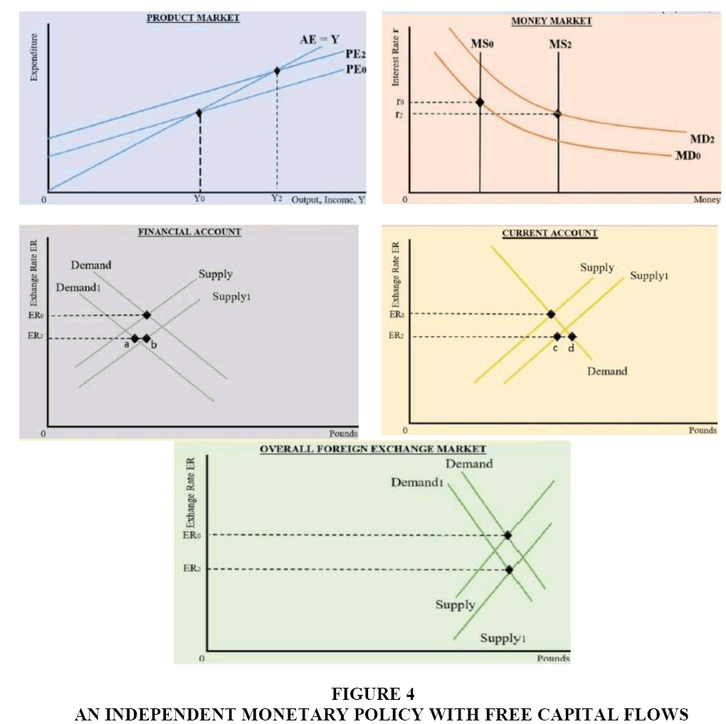
Figure 4: An Independent Monetary Policy with Free Capital Flows
An independent monetary policy and free capital flows are incompatible with exchange rate stability.
As an aside, expansionary monetary policy and free capital flows have an ambiguous effect on imports, since the depreciation reduces imports and the higher income raises imports. Imports could rise enough to more than offset the increase in exports; hence, the effect on the current account is also ambiguous; i.e., it could move into deficit, move into surplus or stay balanced. The effect on the financial account is ambiguous, since any deficit in one account is offset by a surplus in the other account. In Figure 4, the financial account shows deficit of ab pounds, which equals the current account surplus of cd pounds.
Concluding Comments
The present paper complements the paper, “Open Economy Keynesian Macroeconomics without the LM Curve,” by Bajo-Rubio and Diaz-Roldan (2016) in this journal. Their paper analyzes monetary policy under either a flexible exchange rate or a monetary union (not a fixed exchange rate). They observe that the “impossible trilogy,” as they label it, requires policy makers to forgo fixed exchange rates given a desire to pursue monetary policy and allow freedom of capital flows. Hence, they analyze monetary policy under flexible exchange rates using their pedagogical framework. Then building on the work of Obstfeld & Rogoff (1995) and arguing that relatively few countries maintain fixed exchange rates for long periods of time Bajo-Rubio and Diaz-Roldan focus their framework on policies (monetary and fiscal) and macroeconomic shocks on countries belonging to a currency union. The pedagogy in the paper by Bajo-Rubio & Diaz-Roldan is targeted to professors offering courses in Intermediate Macroeconomics. In the present paper, though, the pedagogy is targeted to professors offering courses in International Economics. Note that the model in the present paper can also be used to illustrate the effects of fiscal policy under flexible and fixed exchange rates.
Finally, the other five big ideas that explain how the world works identified by the Economist, in addition to the Mundell-Fleming trilemma, are the Nash equilibrium in game theory, Hyman Minski’s financial instability model, the Stolper-Samuelson international trade theorem on tariffs and wages, George Akerlof’s analysis of asymmetric information in markets and John Maynard Keynes idea on multipliers associated with fiscal policy.
References
- Appleyard, D.R. & Fields Jr., A.J. (2014). International Economics (8th edn). New York, NY: McGraw-Hill, Irwin.
- Bajo-Rubio, O. & Diaz-Roldan, C. (2016). Open economy Keynesian macroeconomics without the LM curve. Journal of Economics and Economic Education Research, 17(2), 1-16.
- Carbaugh, R.J. (2015). International economics (15th edn). Boston, MA: Cengage.
- Daniels, J.P. & Van Hoose, D.D. (2014). International monetary and financial economics. New York, NY: Pearson.
- Dornbusch, R., Fisher, S. & Startz, R. (2014). Macroeconomics (12th edn). New York, NY: McGraw-Hill Irwin. Economist Magazine, The Mundell-Fleming trilemma: Two out of three ain’t bad, (2016, August 27) 1-6.
- Feenstra, R.C. & Taylor, A. (2014). Essentials of international economics (3rd edn). New York, NY: Worth.
- Fleming, J.M. (1962). Domestic financial policies under fixed and under floating exchange rates. International Monetary Fund Staff Papers, 9(3), 369-379.
- Gerber, James (2018). International economics (7th edn). New York, NY: Pearson.
- Hubbard, R.G., O’Brien, A. & Rafferty, M. (2014). Macroeconomics (2nd edn). New York, NY: McGraw-Hill Irwin.
- Husted, S. & Melvin, M. (2013). International economics (9th edn). New York, NY: Pearson.
- Jones, C.I. (2018). Macroeconomics (4th edn). New York, NY: Norton.
- Kreinin, M.E. & Clark, D.P. (2013). International economics (2nd edn). Boston, MA: Pearson.
- Krugman, P.R., Obstfeld, M. & Melitz, M.J. (2015). International economics (10th edn). Boston, MA: Pearson.
- Mankiw, N.G. (2016). Macroeconomics (9th edn). New York, NY: Worth.
- McKinnon, R.I. (1963). Optimum currency areas. American Economic Review, 53(4), 717-725.
- Mishkin, F.S. (2012). Macroeconomics. Boston, MA: Addison-Wesley.
- Mundell, R.A. (1961). A theory of optimum currency areas. American Economic Review. 51(4), 657-665.
- Mundell, R.A. (1962). The appropriate use of monetary and fiscal policy under fixed exchange rates, International Monetary Fund Staff Papers, 9(1), 70-77.
- Mundell, R.A. (1963). Capital mobility and stabilization policy under fixed and flexible exchange rates. Canadian Journal of Economics and Political Science, 9(4), 475-485.
- Obstfeld, M. & Rogoff, K. (1995). The mirage of fixed exchange rates. Journal of Economic Perspectives, 9(4).
- Obstfeld, M & Taylor, A.M. (2017). International monetary relations: Taking finance seriously. Journal of Economic Perspectives, 31(3), 3-28.
- Pugel, T.A. (2016). International economics (16th edn). New York, NY: McGraw Hill.
- Salvatore, D. (2016). International economics (12th edn).Danvers, MA: John Wiley & Sons.
- Sawyer, Charles, W. & Sprinkle, R.L. (2015). Applied international economics (4th edn). London, UK: Routledge.
- Suranovic, S. (2013). International economics. Washington, DC: Flat World Knowledge.
- Thompson, H. (2011). International economics (3rd edn). Singapore: World Scientific Publishing.
- Van Marrewijk, C. (2012). International economics (2nd edn). Oxford, UK: Oxford University Press.
- Yarbrough, B.V. & Yarbrough, R.M. (2006). The world economy: Open-economy macroeconomics and finance (7th edn). Mason, OH: Thomson.