Research Article: 2018 Vol: 22 Issue: 4
A New Perspective on the Cognitive Representation of Internal Reference Price
Rajesh Chandrashekaran, Fairleigh Dickinson University
Keywords
Internal Reference Price, Cognitive Representation, Price Perception.
Introduction
Decades of research have validated that consumer’s evaluations of prices are best explained by invoking the idea that it is driven by some underlying construct that mimics an internal standard of reference commonly referred to as Internal Reference Price, or IRP for short (Cheng and Monroe, 2013). Given the varied definitions of the construct, this article argues that the location (on some mental number line) of the subjective standard against which the individual assesses the selling price as being either “good” or “bad” is not definite. Drawing on revolutionary ideas forwarded by such great physicists as Schrodinger and Heisenberg, this article is based on the idea that individual’s assessments of value of a posted sale price entangled with a subjective fuzzy clouds whose shapes define areas within the clouds where potential internal reference prices are likely to be found. The fundamental premise of this article is that we cannot be certain about the exact location of an individual’s reference price; we can only conjecture about where it might be.
Organization and Contribution
The remainder of this article proceeds as follows: First, a brief review of the literature is presented, focusing specifically on the varied conceptualizations of the construct of internal reference price. Following this, an alternative perspective of the cognitive representation of reference price is presented. Acknowledging that the definition of the construct is a nebulous one, the current research envisions the construct as a random variable existing between upper and lower bounds of price acceptance. Subsequently, results from two studies are presented-each explores a different set of assumptions about the nature of the distribution of reference prices and demonstrates how the specific distributional assumptions (normal versus beta versus triangular) may be used to capture the representation and random retrieval of internal reference prices. In the end, theoretical and practical implications are discussed, along with limitations that could lead to future research.
To the best of the author’s knowledge, this research is the first to consider the possibility that internal reference price may be a randomly accessed variable existing somewhere within a cloud of possibilities that include, but are not limited to, the varied point estimates suggested in previous research. In addition, this research explores several plausible assumptions about the shape of the probability cloud that contains potential reference prices. From a practical perspective, this research may lead to alternative ways of parametrizing consumer choice models that incorporate reference price effects.
Operationalizing Internal Reference Price
An enormous amount of empirical evidence supports the claim that consumers judge sale prices against some subjective Internal Reference Prices (Winer, 1986; Mayhew and Winer, 1992; Kalyanaram and Little, 1994; Briesch et al., 1997). Past research has implemented internal reference price in a multitude of ways.1 For example, Lowengart (2002) identified twenty-six different conceptualizations of reference price. The definitions of IRP include past price (Mayhew and Winer, 1992); average, normal or regular price (Urbany and Dickson, 1991); lowest price (Urbany et al., 1998); lowest market price (Chandrashekaran and Jagpal, 1995); highest price willing to pay or reservation price (Thaler, 1985; Chandrashekaran and Jagpal, 1995); fair price (Thaler, 1985; Lichtenstein and Bearden, 1989); and expected future price (Jacobson and Obermiller, 1990). Interested readers are encouraged to read Cheng and Monore (2013) for an excellent historical perspective of the evolution of research on IRP.
Regardless of how IRP has been operationalized, prior research has most often substituted IRP with a single point estimate for a given individual at a given point in time. However, doing so squishes an entire range of possible reference prices down to a single summary estimate. Furthermore, the dynamic nature of IRP has only been addressed temporally, e.g., by computing it as a moving average over time and across purchase periods. As noted by Cheng and Monroe (2013), “While the empirical indicators that have been used are attempts either to access an individual’s internal reference prices, or to assume buyer’s internal reference prices, we do not have sufficient evidence that these indicators do represent the unobservable construct.”
Cognitive Representation of Reference Price: An Alternate Perspective
The prevailing view of IRP, based on Helson’s Adaptation Level Theory (Helson, 1964) equates the construct to a single point that is best represented by an average (arithmetic or geometric) of previously encountered prices. However, a few researchers (Janiszewski and Lichtenstein, 1999; Neidrich et al., 2001) have pointed out that AL theory does not provide a complete explanation of the cognitive representation of reference price. According to them, the problem with conceptualizing reference price as an adaptation level is that: (a) such a reference is a single point located at somewhere in the middle of a range of prices and (b) it ignores the influences of context on price judgments. Given these limitations, they make a strong and convincing case for alternative theories that may better explain the price judgment process.
For example, Volkman’s (1951) Range Theory argues that the midpoint of the range of previously encountered levels of a stimulus does not hold any special significance. Rather, it is the end points (upper and lower bounds) of the range that drives how a stimulus might be judged. Tversky and Kahneman (1973) have also opined that extreme stimuli are more accessible and easier to retrieve from memory than other points within the range. By manipulating the upper and lower bounds while maintaining the average (internal reference according to AL Theory), Janiszewski and Lichtenstein (1999) successfully demonstrated that changes in price judgments are best explained by changes in the location of the focal price in relation to individual’s lower and upper bounds. Subsequently, Neidrich et al. (2001) provided even stronger evidence to support that range, along with frequency, is an important determinant of how consumers judge a focal price situated within the range.2
Research Objectives
The present research extends previous conceptualizations of IRP by introducing the idea that IRP is a nebulous construct residing merely as probabilities within subjective ranges of price acceptance. The proposed conceptualization theorizes that the likelihood of a particular point serving as a reference price depends on the shape of the probability density function. Such theorizing is consistent with views espoused by Kahneman and Miller (1986), who have suggested that consumers judge stimuli within the context of subjective distributions characterized by a mean, mode and range. The overarching objective of this research is to shed additional light on the cognitive representation of internal reference prices.
Cloudy, With a Chance of IRPS
Despite the general acknowledgement that IRP is likely to fall somewhere within a range and that it may be hard to pinpoint its exact location on a number line, prior research has not envisioned IRP as a random variable for given consumer within a given purchase period. The remainder of this paper is devoted to exploring IRP as a fuzzy, nebulous construct. The underlying assumptions are that: (i) IRP is not a definite point, (ii) it exists merely as a cloud of probabilities within a region of acceptance and (iii) a specific IRP takes life as a random variable from within this cloud at the time of assessing price. Rather than relying solely on the midpoint of the acceptable range of prices to serve as the single most-accurate representation of IRP (as predicted by AL Theory), or only the endpoints of the range (as suggested by Range theory), or any one specific reference price, this study explores the idea that, when faced with a decision, individuals draw IRPs randomly from within subjective probability clouds, using some idiosyncratic rules that define the shapes of the distribution of reference prices within their subjective ranges.
As shown in Figure 1, a multitude of potential reference price (including, but not limited to the ones suggested in prior research) may exist within a large, fuzzy cloud of possibilities. Every price point on the horizontal axis represents a potential IRP that is associated with a subjective probability of being evoked. Consistent with the idea that IRP is a dynamic construct, it assumed that the probabilities (density functions) vary across consumers and over time for the same consumer. In effect, the IRP cloud contains numerous potential reference prices whose exact locations at any given point in time for a given consumer is hard to know-an idea that has not been considered in past research. A fundamental question examined here is: do models using such random IRPs (on average) explain price evaluation better/worse than the standard approach of replacing IRP with midpoint of the range?
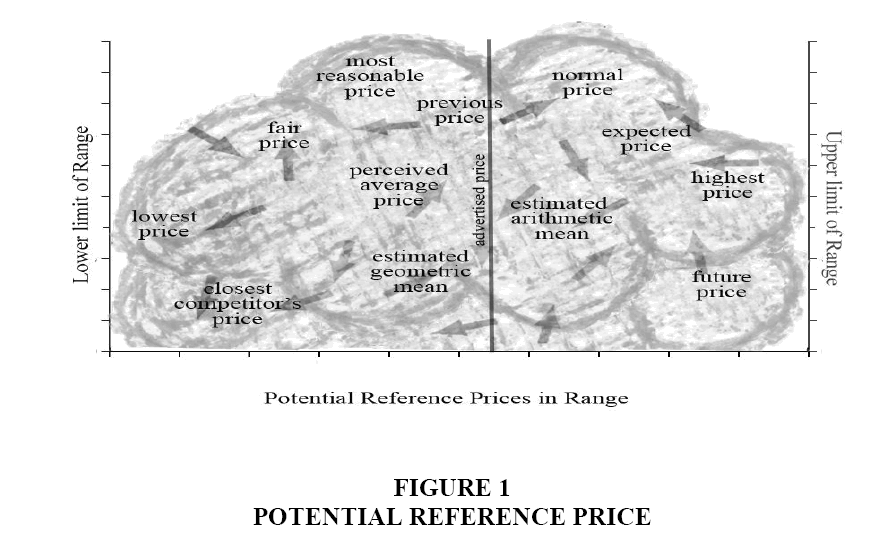
Figure 1: Potential Reference Price
Seeing Shapes in the Clouds
The proposition that IRP exists somewhere within a nebulous probability cloud raises the obvious question regarding the shape of the distribution/cloud. Clearly, there is no basis to assume that: (a) we know the distribution for every individual and that; (b) the distribution is same across all individuals. For starters, addressing the first issue demands that we make reasonable and plausible assumptions regarding the shape of the distribution of IRPs within consumer’s subjective ranges. Three specific probability density functions-Uniform, Standard Normal and the Beta distribution-are explored. In each case, it is assumed that consumers utilize the entire range, including the endpoints defined by individual’s estimates of lowest and highest prices. Additionally, it is assumed that the subjective probability density functions are symmetric about the midpoint of the range (a restriction that is relaxed later).
Uniform distribution: By definition, this assumes that all price points within individual’s acceptable ranges have an equal probability of serving as an IRP against which a posted sale price is evaluated at a particular point in time.
Normal distribution: The assumption that potential reference prices within the range are distributed normally, places the restriction that price points closer to the midpoint (mean/mode) have the highest likelihood of serving as IRPs and the likelihood decreases on either side of the midpoint. Such conceptualization is consistent with AL theory in that significant emphasis is placed on the midpoint (mean) of the range. At the same time, it acknowledges that price points on either side of the midpoint may also serve as references (albeit with lower probabilities).
Beta distribution: This assumption allows for the exploration of two extremes (with appropriate choices of the parameters α and β that define its shape). When α=β=0.5, the maximum values of the symmetric density function are at the endpoints. Such a shape is consistent with the view that the endpoints play crucial roles in determining how a sale price is judged. At the same time, by allowing for other prices in the range to be selected (albeit with very low likelihoods), it deviates from the notion that the endpoints are the sole drivers of price judgments (Figure 2).
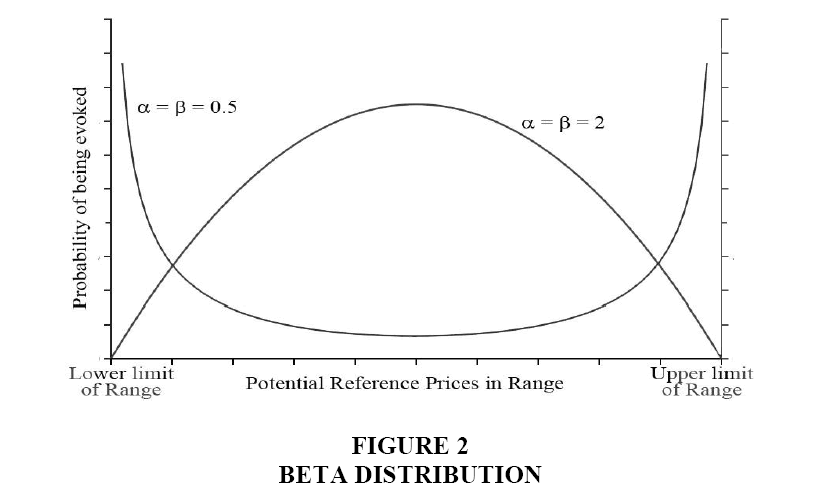
Figure 2: Beta Distribution
Defining α=β=2 yields a distribution that is a reasonable approximation of the normal distribution. Here, the likelihoods of particular points in the range to be used as reference prices is the opposite of when α=β=0.5.3 Specifically, prices in the mid-region of the range have higher probabilities of being evoked compared to those towards the extremes. This specification is consistent with predictions of a somewhat relaxed version of AL Theory.
At first glance, all three distributions are reasonable descriptions of how individuals may behave. For the purposes of this initial exploratory endeavor, it is assumed for the moment that individuals draw their subjective IRPs from similar, but not identically shaped, symmetric distributions-an assumption that is relaxed later in the article. The primary question is whether IRPs drawn randomly from these distributions are better than the standard practice of replacing IRP with the midpoint of the range at explaining consumer’s evaluations of a posted sale price.
Study 1
This objective was to explore how well IRPs drawn randomly from Uniform, Normal and Beta distributions explain consumer’s judgments of price compared to IRPs that are based solely on the midpoint of the range (as implied by AL Theory) and the predictions of Range theory that the endpoints of the range drive price judgments.
Study 2
Following three carefully planned experiments to demonstrate the superiority of Range-Frequency theory over Adaptation Level and Range theories, Niedrich et al. (2001) concluded that, “Consumers not only have a sense of the range but also of the relative frequencies of prices they have encountered.” To explore the veracity of that assertion in the context of IRP clouds, Study 2 elicited subjective estimates of price points within individual’s ranges that represented their estimates of the most frequent or most reasonable prices for the product. This information, along with estimates of lower and upper limits of subjective ranges, allows for the incorporation of positive/negative skew in individual distributions. Three possibilities (in addition to the single reference model predicted by AL theory) were considered: a biased normal distribution, a biased beta distribution and a triangular distribution (discussed later).
Methodology
Study 1
Eighty business majors participated in an online study that consisted of three stages (Note: six subjects were discarded because they failed to complete a major portion of the survey). First, participants saw a picture of a fictitious brand of backpack along with a list of the product’s features, but without any price information. After studying the information, participants provided estimates of highest price they are willing to pay and the lowest acceptable price at which they are likely to just start doubting the quality of the product. Immediately following this, subjects completed a couple of distraction tasks (e.g., mentally manipulating and matching shapes) intended to clear out contents of working memory. Finally, participants were shown the same advertisement they had seen previously, but with a selling price ($29.92) included. This price point was selected based on an examination of the undiscounted prices of similar backpacks available at major retail outlets, the college’s bookstore and at popular online sites. After scrutinizing the ad, subjects evaluated the Perceived Offer Value (POV), which was assessed using four 7-point scale items related to: attractiveness of the deal, value for money, purchase intention and the likelihood of finding a lower price (Grewal et al., 1998).
Factor analysis of the six items (two related to IRP and four related to offer value) confirmed a two factor solution explaining a total of 78% of the variance, with the items related IRP and POV loading on separate factors. In addition, the scales created by the respective measures were highly reliable (Correlation between IRP measures=0.89 and Chronbach’s alpha for POV scale=0.87). Based on this, IRP and POV were computed as the arithmetic averages of their respective proxies.
Study 2
Ninety-five undergraduate students participated in this study. The method employed was exactly the same as that employed in Study 1 except that, in Part 1, respondents also provided information on their estimates of what they considered to be the most reasonable (most frequently encountered) price for the product. The estimates of the most reasonable prices served as the modes of the subjective distributions that introduce systematic biases (skewness) in the generation of IRPs from subjective IRP clouds.
Biased Normal and Beta Distributions
For each individual, a systematic bias in generation of random IRP was introduced by shifting the entire distribution in the direction of the subjective or perceived midpoint of the range (i.e., individual estimates of the most reasonable price for the product) and truncating it at the endpoints corresponding to lower and upper bounds of the range (Figure 3).
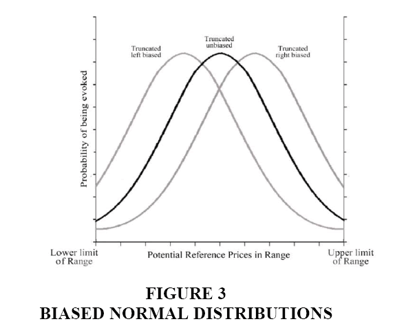
Figure 3: Biased Normal Distributions
In effect, the mean of the new (normal) distribution shifts to the perceived midpoint of the range. Although it does not technically skew the subjective distributions (in the strict, statistical definition of the term), shifts in the means of the subjective distributions along with the truncation at the endpoints introduces asymmetries in the distributions within the subjective ranges that biases the random generation of IRPs in the direction of the shift (i.e., in the direction of the subjective estimates of the most reasonable price for the product).
A similar procedure was employed to skew the subjective beta distributions, except that in this case, the distribution was stretched in the direction of the most reasonable price by an amount equal to the difference between the midpoint of the range and the most reasonable price estimate. Finally, the distribution was truncated as required to ensure that evoked IRPs came from within the range (Figure 4).
The Triangular Distribution
This distribution has been shown to be a good proxy for other, more sophisticated distributions like the normal and the beta distributions (Johnson, 1997). The appeal of the triangular distribution is that it is simple, versatile and it offers the flexibility to capture an array of skewed triangles based on the particular point at which the mode occurs. For example, when the mode of the distribution corresponds to the lower limit of the range, the density function resembles a left-armed right triangle. Similarly, when individuals place most emphasis on the upper limit the density function resembles a right-armed right triangle. It is easy to see that, by varying the point at which the mode occurs, the density function is able to capture differently shaped triangles across the gamut.
In this way, a triangular distribution allows for the incorporation of some heterogeneity in the shape of distribution of potential reference prices. The triangular distribution is particularly useful when the limits (upper and lower) are known and a most likely value in the range is known, but the exact nature of the distribution is unknown-a scenario that is quietly likely in the context of IRPs. Given these three pieces of information, it is possible to create a wide array of skewed distributions within a given range by simply varying the coordinates of the mode.
As shown in Figure 5, if ‘u’ and ‘l’ represent the upper and limits of the range and ‘m’ represents the mode (i.e., estimate of the most likely value) and R is a random number generated from a uniform distribution bounded by (0, 1), then a random variable X from a triangular distribution bounded by [l, u] can be expressed as:
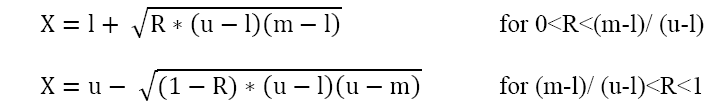
Such a distribution is particularly suitable in the context of internal reference prices because it is often easy to deduce, estimate, or measure the three points (lowest price, highest price and price encountered most often) that are sufficient to generate a triangular probability density function. The distribution is both intuitive and versatile in that it allows us to incorporate individual differences with respect to the shape (i.e., skewness) of the distribution depending on subjective values of m (most reasonable price) in relation to l (lower limit), u (upper limit).
Results
Study 1
The final analysis included 74 respondents. The intent was to compare how randomly generated IRPs compare against the more traditional approach.
The traditional model: Per AL Theory, both arithmetic and geometric means of upper and lower points of the range (high but willing and low enough to not doubt the quality) served as substitutes for IRP in two separate analyses. Consistent with Prospect Theory (Kahneman and Tversky, 1979), perceived Gain and Loss terms were specified based on the extent and direction of the deviation of the posted sale price from each IRP separately.
Gain=IRP-Sale Price if IRP>Sale Price; 0 if IRP<Sale Price.
Loss=|IRP-Sale Price| if IRP<Sale Price; 0 if IRP>Sale Price.
In two separate analyses (one using the arithmetic mean and another using the geometric mean), the dependent variable (POV) was regressed on Gain and Loss. Overall, both models fit the data reasonably well (F=40.76, p<0.001, R2=0.55 for arithmetic mean model; and F=42.11, p<0.001, R2=0.54 for the geometric mean model). As predicted by Prospect Theory (Kahneman and Tversky, 1979), respondents are significantly more sensitive to losses (βloss= -0.11, t= -6.48, p<0.001 for the both models) than they are to gains (βgain=0.05, t=3.10, p<0.01 for the arithmetic model and βgain=0.04, t=2.47, p<0.05 for the geometric mean model). In summary, the results obtained here reconfirm that IRP is a valuable construct in explaining how consumers evaluate retail prices and that responses to deviations in price on either of the reference point are not symmetric.
Endpoints as IRPs: To ascertain whether IRPs based on the endpoints are capable of explaining consumer’s evaluations of price, POV was regressed against Gain and Loss computed based on the extent to which the sale price deviated from each of the endpoints (upper and lower limits of the range). The model using deviations of sale price from individual’s upper limits fit the data well (F=68.02, p<0.001; R2=0.51 and Adjusted R2=0.49). Additionally, the estimated parameters were consistent with the expectation that perceived losses loom larger than perceived gains (βgain=0.05, t=5.09; and βloss= -0.08, t=-3.80).
Exploring the idea of IRP as a random variable: First, width of subjective price range was computed as the numerical difference between the highest and lowest price estimates provided. The next step involved making assumptions about individual’s IRP probability clouds within their subjective ranges. Four possible distributions were considered: uniform, standard normal and two types of beta distributions (with shape parameters α=β=0.05 and α=β=2). Given the exploratory nature of this study, no a priori expectations are offered in terms of which assumption yields the best representation of IRP.
The same procedure was employed in each of the four cases:
1. For all participants, generate random IRPs from subjective ranges defined by [lower limit, upper limit].
2. Compute Gain and Loss terms based on extent and direction of deviation of sale price from the randomly evoked IRPs.
3. Regress POV on the Gain and Loss terms.
4. Repeat steps 1-3 one hundred times.
IRPs from a uniform distribution: Table 1 shows a sample of the results from the first thirty runs. The average R2 value from all of the one hundred regressions was 0.43 (std. dev=0.05) and the means of the parameter estimates βgain and βloss were 0.04 and -0.08 respectively.
| Table1 Sample Results From Study 1 (Irps Drawn From Uniform And Normal Distributions) |
||||||
| Run | IRPs drawn from Subjective Uniform Distributions | IRPs drawn from Subjective Normal Distributions |
||||
| 1 | R2 | βgain | βloss | R2 | βgain | βloss |
| 2 | 0.43 | 0.04 | -0.08 | 0.54 | 0.04 | -0.11 |
| 3 | 0.46 | 0.05 | -0.09 | 0.46 | 0.05 | -0.09 |
| 4 | 0.38 | 0.04 | -0.08 | 0.48 | 0.04 | -0.10 |
| 5 | 0.41 | 0.04 | -0.08 | 0.49 | 0.04 | -0.11 |
| 6 | 0.33 | 0.04 | -0.07 | 0.43 | 0.05 | -0.08 |
| 7 | 0.39 | 0.04 | -0.08 | 0.53 | 0.04 | -0.10 |
| 8 | 0.39 | 0.03 | -0.08 | 0.42 | 0.05 | -0.09 |
| 9 | 0.4 | 0.05 | -0.06 | 0.51 | 0.05 | -0.09 |
| 10 | 0.51 | 0.04 | -0.09 | 0.54 | 0.04 | -0.11 |
| 11 | 0.32 | 0.05 | -0.06 | 0.53 | 0.04 | 0.11 |
| 12 | 0.39 | 0.04 | -0.08 | 0.54 | 0.04 | -0.10 |
| 13 | 0.46 | 0.04 | -0.1 | 0.51 | 0.03 | -0.11 |
| 14 | 0.48 | 0.04 | -0.09 | 0.50 | 0.04 | -0.10 |
| 15 | 0.48 | 0.05 | -0.08 | 0.51 | 0.05 | -0.10 |
| 16 | 0.5 | 0.04 | -0.09 | 0.45 | 0.05 | -0.08 |
| 17 | 0.37 | 0.03 | -0.08 | 0.49 | 0.04 | -0.10 |
| 18 | 0.47 | 0.05 | -0.08 | 0.50 | 0.05 | -0.09 |
| 19 | 0.48 | 0.05 | -0.08 | 0.45 | 0.05 | -0.09 |
| 20 | 0.43 | 0.05 | -0.08 | 0.51 | 0.04 | -0.10 |
| 21 | 0.4 | 0.05 | -0.08 | 0.46 | 0.04 | -0.09 |
| 22 | 0.41 | 0.03 | -0.09 | 0.48 | 0.04 | -0.10 |
| 23 | 0.45 | 0.04 | -0.08 | 0.49 | 0.05 | -0.10 |
| 24 | 0.42 | 0.03 | -0.09 | 0.47 | 0.04 | -0.09 |
| 25 | 0.52 | 0.04 | -0.09 | 0.48 | 0.04 | -0.10 |
| 26 | 0.5 | 0.05 | -0.1 | 0.50 | 0.06 | -0.09 |
| 27 | 0.36 | 0.05 | -0.08 | 0.51 | 0.04 | -0.11 |
| 28 | 0.46 | 0.03 | -0.1 | 0.48 | 0.05 | -0.08 |
| 29 | 0.43 | 0.03 | -0.09 | 0.48 | 0.06 | -0.09 |
| 30 | 0.46 | 0.05 | -0.08 | 0.54 | 0.04 | -0.11 |
Table 1, results from the first 30 regression analyses of POV against Gain and Loss for models with IRPs drawn randomly from subjective Uniform and Normal distributions. R2 is the proportion of variation in the dependent variables explained by the independent variables Gain and Loss; and βgain and βloss are the estimated parameters for the Gain and Loss terms respectively.
Although models using IRPs drawn randomly from uniformly distributed probability density functions explain a reasonable proportion of the variation in POV (mean R2=43%), they underperform in comparison with the traditional model that explained a significantly higher percentage (55%) of the variation in POV.
Normally distributed IRPs: Potential IRPs were drawn randomly from subjective, symmetric normal distributions with means specified as the midpoints of the subjective ranges and standard deviations estimated based on the assumption that, for each individual, the lower and upper limits represent the 1st and the 99th percentiles of their subjective distribution. The randomly generated IRPs were truncated at the subjective upper and lower limits so that all IRPs came from within the subjective regions of acceptance. For each of the one hundred regressions, Gain and Loss terms served as independent variables and POV served as the dependent variable.
Table 1 contains a sample of the results of the first thirty (out of one hundred) runs. On average, IRPs drawn from a normally distributed pdf explained 49% of the variation in POV and the mean parameters estimates βgain and βloss were 0.04 and -0.08 respectively. It is interesting to note that the parameter estimates βgain and βloss are exactly the same (rounded to the second decimal) as those obtained from the analysis using uniformly distributed IRPs. Although significant, the proportion of the variation in POV explained here falls short of that explained by the traditional model.
IRPs drawn from Beta distributions: As seen in Table 2, two alternatives were considered. The first (with α=β=0.5) places major emphasis on the endpoints of the range, whereas the second (with α=β=2) favors IRPs close to the midpoint of the range. The resulting shape is a reasonable approximation of a normal curve, without requiring truncation because this type of beta distribution truncates naturally at the endpoints.
| Table 2 Sample Results From Study (Irps Drawn From Beta Distributions) |
||||||
| Run# | IRPs drawn from Subjective Beta Distributions (with α=β=0.5) | IRPs drawn from Subjective Beta Distributions (with α=β=2) | ||||
| R2 | βgain | βloss | R2 | βgain | βloss | |
| 1 | 0.47 | 0.05 | -0.09 | 0.41 | 0.05 | -0.07 |
| 2 | 0.42 | 0.06 | -0.07 | 0.49 | 0.04 | -0.10 |
| 3 | 0.40 | 0.04 | -0.07 | 0.49 | 0.06 | -0.09 |
| 4 | 0.45 | 0.03 | -0.09 | 0.49 | 0.04 | -0.10 |
| 5 | 0.43 | 0.04 | -0.07 | 0.47 | 0.04 | -0.10 |
| 6 | 0.41 | 0.05 | -0.07 | 0.5 | 0.05 | -0.09 |
| 7 | 0.34 | 0.03 | -0.08 | 0.56 | 0.05 | -0.09 |
| 8 | 0.35 | 0.04 | -0.08 | 0.54 | 0.05 | -0.10 |
| 9 | 0.37 | 0.05 | -0.06 | 0.48 | 0.05 | -0.08 |
| 10 | 0.32 | 0.04 | -0.07 | 0.39 | 0.05 | -0.08 |
| 11 | 0.38 | 0.04 | -0.09 | 0.42 | 0.05 | -0.09 |
| 12 | 0.41 | 0.04 | -0.08 | 0.5 | 0.04 | -0.11 |
| 13 | 0.41 | 0.03 | -0.09 | 0.52 | 0.05 | -0.10 |
| 14 | 0.31 | 0.04 | -0.07 | 0.43 | 0.04 | -0.09 |
| 15 | 0.49 | 0.04 | -0.08 | 0.5 | 0.04 | -0.10 |
| 16 | 0.47 | 0.03 | -0.09 | 0.42 | 0.05 | -0.09 |
| 17 | 0.42 | 0.04 | -0.08 | 0.52 | 0.03 | -0.11 |
| 18 | 0.50 | 0.04 | -0.10 | 0.44 | 0.04 | -0.09 |
| 19 | 0.42 | 0.05 | -0.07 | 0.44 | 0.05 | -0.08 |
| 20 | 0.48 | 0.05 | -0.09 | 0.49 | 0.04 | -0.11 |
| 21 | 0.48 | 0.04 | -0.09 | 0.52 | 0.04 | -0.10 |
| 22 | 0.39 | 0.05 | -0.08 | 0.47 | 0.04 | -0.10 |
| 23 | 0.38 | 0.03 | -0.08 | 0.5 | 0.04 | -0.09 |
| 24 | 0.51 | 0.04 | -0.09 | 0.48 | 0.05 | -0.09 |
| 25 | 0.40 | 0.03 | -0.10 | 0.44 | 0.06 | -0.08 |
| 26 | 0.42 | 0.04 | -0.08 | 0.43 | 0.04 | -0.08 |
| 27 | 0.47 | 0.04 | -0.09 | 0.44 | 0.05 | -0.08 |
| 28 | 0.43 | 0.03 | -0.09 | 0.37 | 0.04 | -0.07 |
| 29 | 0.38 | 0.04 | -0.08 | 0.52 | 0.05 | -0.10 |
| 30 | 0.43 | 0.03 | -0.10 | 0.47 | 0.03 | -0.10 |
Table 2 contains sample results of regressing POV on Gain and Loss terms computed using IRPs drawn from the two beta distributions.
In Table 2, results from the first 30 regression analyses of POV against Gain and Loss for models with IRPs drawn randomly from subjective Beta distributions with different shape parameters. R2 is the proportion of variation in the dependent variables explained by the independent variables Gain and Loss; and βgain and βloss are the estimated parameters for the Gain and Loss terms respectively. On average, IRPs drawn from a beta distribution favoring the middle of the range explained a significantly higher proportion of the variation in POV than one emphasizing the endpoints (49% vs. 41%). In both cases, parameter estimates were as expected and in the same range as those obtained with the other models.5
Study 2
The first step was to estimate the baseline, i.e., the Traditional Model. For this, individuals’ IRPs were computed as the midpoints of their subjective price ranges and POV for each individual was computed as the average of four 7-point scale items. Gain and Loss terms were specified as done in Study 1 (i.e., based on the magnitude and direction of the deviation of IRP from the posted sale price). As in Study 1, two sets of IRPs were used-one computed as the arithmetic mean of the upper and lower limits and the other computed as the geometric mean of the endpoints.
Results from the two regression analyses with POV as the dependent variable reveal that both models (arithmetic and geometric) reveal that both models fit the data well (F=19.92, p<0.001 for the arithmetic mean model and F=20.07, p<0.001 for the geometric mean model). In both cases, the independent variables (i.e., Gain and Loss) explained a similar proportion of the variation in POV (R2=0.30, Adjusted R2=0.29).6 as expected, perceived gains enhance POV and perceived losses depress POV. Finally, consistent with the predictions of Prospect Theory (Kahneman and Tversky, 1979), respondents appeared more sensitive to losses than to equivalent gains (βgain=0.03, t=2.12, p<0.05; βloss=-0.13, t=-3.88, p<0.001 for the arithmetic mean model and βgain=0.03, t=1.88, p<0.10; βloss=-0.12, t=-3.95, p<0.001 for the geometric mean model).
IRPs from biased normal distributions: As before, a total of one hundred regressions were run using POV as the dependent variable and Gain and Loss terms as the independent variables. Table 3 contains a sample of the results from the first thirty runs. It is clear that, on average, the mean proportion of variation explained by this model is significantly higher than that explained by the Traditional model (Mean R2biased normal=0.41, R2traditional=0.30).
| Table 3 Sample of Results From Study 2 |
|||||||||
| Run# | IRPs from Subjective Biased Normal Distributions | IRPs from Subjective Biased Beta Distributions | IRPs drawn from Subjective Triangular Distributions | ||||||
| R2 | βGain | βLoss | R2 | βGain | βLoss | R2 | βGain | βLoss | |
| 1 | 0.45 | 0.04 | -0.14 | 0.43 | 0.03 | -0.14 | 0.40 | 0.06 | -0.11 |
| 2 | 0.39 | 0.04 | -0.13 | 0.36 | 0.01 | -0.15 | 0.41 | 0.02 | -0.15 |
| 3 | 0.4 | 0.03 | -0.14 | 0.30 | 0.02 | -0.13 | 0.47 | 0.03 | -0.15 |
| 4 | 0.44 | 0.02 | -0.14 | 0.22 | 0.03 | -0.09 | 0.38 | 0.06 | -0.10 |
| 5 | 0.44 | 0.03 | -0.15 | 0.33 | 0.00 | -0.15 | 0.38 | 0.04 | -0.13 |
| 6 | 0.48 | 0.18 | -0.17 | 0.32 | 0.01 | -0.15 | 0.46 | 0.04 | -0.14 |
| 7 | 0.41 | 0.02 | -0.15 | 0.29 | 0.03 | -0.10 | 0.41 | 0.05 | -0.12 |
| 8 | 0.40 | 0.04 | -0.13 | 0.21 | 0.02 | -0.10 | 0.42 | 0.04 | -0.13 |
| 9 | 0.40 | 0.03 | -0.13 | 0.34 | 0.l04 | -0.10 | 0.53 | 0.02 | -0.17 |
| 10 | 0.46 | 0.05 | -0.13 | 0.34 | 0.04 | -0.12 | 0.43 | 0.03 | -0.13 |
| 11 | 0.45 | 0.02 | -0.16 | 0.29 | 0.04 | -0.10 | 0.39 | 0.04 | -0.12 |
| 12 | 0.43 | 0.03 | -0.14 | 0.30 | 0.05 | -0.09 | 0.47 | 0.04 | -0.14 |
| 13 | 0.44 | 0.04 | -0.13 | 0.28 | 0.02 | -0.13 | 0.41 | 0.02 | -0.15 |
| 14 | 0.44 | 0.04 | -0.14 | 0.26 | 0.01 | -0.13 | 0.49 | 0.04 | -0.14 |
| 15 | 0.42 | 0.03 | -0.14 | 0.34 | 0.01 | -0.14 | 0.43 | 0.03 | -0.14 |
| 16 | 0.37 | 0.05 | -0.12 | 0.32 | 0.03 | -0.12 | 0.38 | 0.05 | -0.11 |
| 17 | 0.48 | 0.04 | -0.16 | 0.34 | 0.04 | -0.11 | 0.43 | 0.03 | -0.14 |
| 18 | 0.41 | 0.03 | -0.14 | 0.31 | 0.01 | -0.13 | 0.46 | 0.04 | -0.15 |
| 19 | 0.40 | 0.04 | -0.13 | 0.28 | 0.04 | -0.11 | 0.41 | 0.02 | -0.14 |
| 20 | 0.44 | 0.04 | -0.13 | 0.33 | 0.03 | -0.12 | 0.34 | 0.04 | -0.11 |
| 21 | 0.42 | 0.04 | -0.14 | 0.33 | 0.01 | -0.14 | 0.42 | 0.03 | -0.13 |
| 22 | 0.40 | 0.04 | -0.14 | 0.26 | 0.01 | -0.13 | 0.43 | 0.02 | -0.15 |
| 23 | 0.40 | 0.02 | -0.15 | 0.30 | 0.05 | -0.10 | 0.38 | 0.05 | -0.11 |
| 24 | 0.47 | 0.03 | -0.16 | 0.26 | 0.05 | -0.08 | 0.40 | 0.03 | -0.12 |
| 25 | 0.39 | 0.04 | -0.13 | 0.26 | 0.04 | -0.09 | 0.46 | 0.04 | -0.14 |
| 26 | 0.47 | 0.04 | -0.14 | 0.36 | 0.02 | -0.14 | 0.36 | 0.06 | -0.11 |
| 27 | 0.41 | 0.03 | -0.14 | 0.27 | 0.03 | -0.09 | 0.49 | 0.03 | -0.15 |
| 28 | 0.33 | 0.03 | -0.13 | 0.29 | 0.02 | -0.13 | 0.45 | 0.04 | -0.14 |
| 29 | 0.40 | 0.03 | -0.14 | 0.30 | 0.02 | -0.12 | 0.47 | 0.06 | -0.12 |
| 30 | 0.40 | 0.03 | -0.14 | 0.27 | 0.03 | -0.12 | 0.46 | 0.03 | -0.14 |
In Table 3, results from the first 30 regression analyses of POV against Gain and Loss for models with IRPs drawn randomly from subjectively biased normal, beta and triangular distributions. R2 is the proportion of variation in the dependent variables explained by the independent variables Gain and Loss; and βgain and βloss are the estimated parameters for the Gain and Loss terms respectively.
IRPs from biased beta distributions: Sample of results from the first thirty runs using randomly generated IRPs from biased beta distributions (with shape parameters α=β=2) are shown in Table 2. On average, these IRPs explained about the same proportion of the variation in POV as did the traditional models (R2=0.31 for the beta distribution model versus R2=0.30 for the arithmetic and geometric mean models).
IRPs from a triangular distribution: For each subject, subjective triangular distributions were created, IRPs were drawn randomly. As before, one hundred regressions were run using POV as the dependent variable and Gain and Loss terms corresponding to the deviation between the randomly generated IRPs and the posted sale price. Table 2 contains sample results from the first thirty (of one hundred) regressions. On average, IRPs drawn from a triangularly distributed IRP cloud explained 43% of the variation in the dependent variable, POV. This is significantly better than the proportion of variation in POV explained by the traditional model and, on average, moderately better than the biased normal distribution models (R2triangular=0.43, R2biased-normal=0.41, R2traditional=0.30).
General Discussion
This research offered a radically different perspective on the cognitive representation of IRP. Breaking away from the traditional conceptualization of IRP as a single, well-defined price for a given individual at a given point in time, this research introduced the notion of a nebulous probability cloud bounded by upper and lower limits and containing many probable references. Study 1 compared three reasonable probability density distribution functions-uniform, standard normal and beta. Although the models explained satisfactory proportions of the variation in the dependent variable, they did not outperform the traditional approach of defining IRP as the (arithmetic or geometric) mean of prices within consumer’s subjective ranges.
Study 2 went a step further by introducing skewness in the shapes of the subjective distributions. This was accomplished by including estimates of the most reasonable price to serve as proxies for the modes of the subjective density functions. Again, three possibilities were considered. The first was a biased normal distribution created by shifting the entire distribution in the direction of the most reasonable price to skew the probabilities with which IRPs are drawn from subjective IRP clouds. The second was a biased beta distribution and the third was a novel and yet intuitive triangular distribution, which has been applied in the analysis of risk and has been shown to be a good substitute for more complex distributions. Most importantly, the three pieces of information required to calibrate this density function (upper limit, lower limit and most likely value) are directly related to the formation of reference prices. Results from both these models (biased normal and triangular) outperformed the traditional model by explaining a significantly higher proportion of the variation in the dependent variable. Table 4 summarizes results from both studies.
| Table 4 Comparison of Alternative Operationalization of IRP From Study 1 And Study 2 |
||||||
| IRP operationalized as: | Study 1 (n=74) Symmetric Distributions |
Study 2 (n=96) | ||||
| (mean) R2 | βgain | βloss | (mean) R2 | βgain | βloss | |
| Arithmetic mean of upper and lower limits of range | 0.55 | 0.05 | -0.11 | 0.30 | 0.03 | -0.13 |
| Geometric Mean of upper and lower limits of range | 0.54 | 0.04 | -0.11 | 0.30 | 0.03 | -0.12 |
| Lower Limit of Price Range | Not estimated because of very few “Gain” terms. | 0.28 | 0.02† | -0.11 | ||
| Upper Limit of Price Range | 0.51 | 0.05 | -0.08 | Not estimated because of very few “Loss” terms. | ||
| RV from Uniform Distributions | 0.43 | 0.04 | -0.08 | 0.26 | 0.03 | -0.09 |
| RV from Beta Distributions (with α=β=0.5)‡ | 0.41 | 0.04 | -0.08 | Models using these unbiased/symmetric distributions were not estimated in Study 2. | ||
| RV from Beta Distributions (with α=β=2) ‡ | 0.49 | 0.05 | -0.09 | |||
| RV from Normal Distributions‡ | 0.49 | 0.04 | -0.08 | 0.28 | 0.03 | -0.12 |
| RV from Biased Normal Distributions‡ | Not estimated in Study 1 due to lack of appropriate data. | 0.41 | 0.04 | -0.14 | ||
| RV from Biased Beta Distributions (α=β=2) ‡ | 0.31 | 0.03 | -0.12 | |||
| RV from Triangular Distributions | 0.43 | 0.04 | -0.13 | |||
Note: †Not significant (p>0.10); ‡Mean values based on a total of 100 regressions.
In Table 4 the comparison of results from Studies 1 and 2 using different operationalizations of IRP. R2 is the proportion of variation in the dependent variables explained by the independent variables Gain and Loss; and βgain and βloss are the estimated parameters for the Gain and Loss terms respectively.
Conclusion
Study 1
Findings from Study 1 appear to favor an AL theory account of reference price even when prices from the entire range are incorporated in the IRP generation process. However, this conclusion might be premature because all models (normal and beta distribution models) were restricted to be symmetric about the midpoint. In reality, it is likely that individual’s subjective distributions are skewed. For example, it is likely that subjective distributions from which consumers draw IRPs are biased in the direction of the most frequently encountered prices (or the most reasonable price) within the range. Such an explanation is consistent with Range-Frequency theory (Neidrich et al., 2001).
Limitation
Study 1: measured only upper and lower limits of participant’s price acceptance ranges. Although the information allowed for some exploration of alternative distributions (uniform, normal and beta) within this range, it did not facilitate educated guesses about the skewness of the subjective distributions that would have introduced another dimension of heterogeneity.
Study 2: explored relatively simple and intuitive ways of investigating how consumers might draw IRPs from within their (biased) subjective ranges of price acceptance. A novel inclusion was the triangular distribution, which has not been examined in the context of how consumers evaluate prices. Overall, incorporating subjective bias in IRP generation yields results that are significantly better than traditional methods of operationalizing IRP. The findings support the idea that both range and frequency influence internal standards that are evoked when judging prices.
Relevance and Future Research
This research forwarded the notion that IRPs may exist as random variables within nebulous, subjective probability clouds and presented a systematic investigation of distribution types from which individuals draw IRPs. It also introduced the flexible and intuitive triangular density function, which is particularly suited in this context. The three points of information required to define it (highest, lowest and most frequently occurring values) are relatively easy to estimate from scanner data. From a practical perspective, further research on the topic could lead to alternative ways of parametrizing consumer choice models incorporating reference price effects.
Limitation
While this research made some reasonable assumptions regarding the shapes of subjective IRP clouds, there are other possible density functions that could be tested. Candidates include Semi-circular, Cosine and Weibull distributions. Future research may be able to segment consumers based on the shapes of their distributions and to identify individual level factors that may better predict which individuals are likely to draw IRPs from specific distributions.
It is hoped that this initial exploratory investigation will urge more research on the topic that will yield to a much better understanding of the hitherto elusive construct.
Footnotes
1. It must be noted that, while IRP is an individual level construct, store-level panel data typically contains a history of purchases made by the household and may not be reflective of any one individual’s response pattern.
2. Many thanks to David Hardesty for commenting on an early draft of the manuscript and for drawing my attention to Range and Range-Frequency theories.
3. It is quite likely that the shape parameters α and β vary across consumers. Although the exact estimation of individual shape parameters is outside the scope of this exploratory endeavor, it may be an interesting avenue for future empirical research. Estimation of individual’s shape parameters may be used to group into segments according to the values of these shape parameters. However, such analysis is outside the immediate scope of this research.
4. Unfortunately, the model using the lower limit could not be estimated because of a very small number of non-zero Gain terms.
5. On average, the model generating IRPs from a beta distribution with α=β=2 explains the same proportion of variation (R2=0.49, rounded to the second decimal) in POV as the one that drew IRPs from a normal distribution. This result lends some support to the claim that such a beta distribution may be a reasonable approximation of a normal distribution.
6. It is surprising that the F-value and R2 obtained in Study 1 are unusually larger than those obtained in Study 2. One possible explanation could be that Study 1 was conducted relatively early in the academic year, when students are likely to have searched for and/or purchased backpacks for the upcoming year. It is our conjecture that students participating in Study 1 may have possessed greater knowledge of prices than those who participated in Study 2, which was conducted in the second half of the academic year. Unfortunately, we did not gather data on subjective estimates of price and/or product knowledge. A second notable difference is that respondents in Study 1 consisted of senior undergraduate and graduate students, whereas the data for Study 2 came exclusively from undergraduate students (primarily sophomores). Regardless of this, it is important to note that this research makes comparisons across alternative distributional assumptions within each study and not across studies. Therefore, we do not believe that the conclusions would have been any different.
References
- Briesch, R.A., Krishnamurthi, L, Mazumdar, T, & Raj, S.P. (1997). A comparative analysis of reference price models. Journal of Consumer Research, 24(2), 202-214.
- Chandrashekaran, R., & Harsharanjeet, J. (1995). Is there a well-defined reference price? In Advances in Consumer Research, 22(1), 230-235.
- Cheng, L.L., & Kent, B.M. (2013). An appraisal of behavioral price research (Part1): Price as a physical stimulus. AMS Review, 3(3), 103-129.
- Grewal, D., Monroe, K.B., & Krishnan, R. (1998). The effects of price comparison advertising on buyers’ perceptions of acquisition value, transaction value, and behavioral intentions. Journal of Marketing, 62(2), 46-59.
- Helson, H. (1964). Adaptation-level theory: An experimental and systematic approach to behavior, (First Edition). New York, NY: Harper & Row.
- Jacobson, R., & Carl, O. (1990). The formation of expected future price: A reference price for forward-looking consumers. Journal of Consumer Research, 16(4), 420-432.
- Janiszewski, C., & Donald, R.L. (1999). A range theory account of price perception. Journal of Consumer Research, 24(4), 353-368.
- Johnson, D. (1997). The Triangular distribution as a proxy for the beta distribution in risk analysis. Journal of the Royal Statistical Society, 46(3), 387-398.
- Kahneman, D., & Amos, T. (1979). Prospect theory: An analysis of decisions under risk. Econometrika, 47(1), 262-291.
- Kahneman, D., & Dale, T.M. (1986). Norm theory: Comparing reality to its alternatives. Psychological Review, 93(2), 136-153.
- Kalyanaram, G., & John, D.C.L. (1994). An empirical analysis of latitude of price acceptance in consumer packaged goods. Journal of Consumer Research, 21(6), 408-418.
- Lichtenstein, D.R., & William, O.B. (1989). Contextual influences on perceptions of merchant-supplied reference prices. Journal of Consumer Research, 16(1), 55-66.
- Lowengart, O. (2002). Reference price conceptualizations: An integrative framework of analysis. Journal of Marketing Management, 18(2), 145-171.
- Mayhew, G.E., & Russell, S.W. (1992). An empirical analysis of internal and external reference prices using scanner data. Journal of Consumer Research, 19(5), 62-70.
- Niedrich, R.W., Sharma, S., & Doudlas, H.W. (2001). Reference price and price perceptions: A comparison of alternative models. Journal of Consumer Research, 28(6), 339-354.
- Thaler, R. (1985). Mental accounting and consumer choice. Marketing Science, 4(1), 199-214.
- Tversky, A., & Kahneman, D.(1973). Availability: A heuristic for judging frequency and probability. Cognitive Psychology, 5(1), 207-232.
- Urbany, J.E., & Peter, R.D. (1991). Consumer normal price estimation: market vs. personal standards. Journal of Consumer Research, 17(4), 45-51
- Volkmann, J. (1951). Scales of judgment and their implications for social psychology. In Social Psychology at the Crossroads, 14(3) 273-294.
- Winer, R. (1986). A reference price model of brand choice for frequently purchased products. Journal of Consumer Research, 13(6), 250-256