Research Article: 2026 Vol: 30 Issue: 4
An Explainable Machine Learning Framework for Predicting NIFTY 50 Stock Market Direction Using XGBoost and SHAP Analysis.
Rajendra Prasada Sabat, Research Scholar. Sri Sri University, Cuttack, Odisha, India
Sudhanshu Sekhar Nanda,Associate Professor Sri Sri University, Cuttack, Odisha
Biplab Kumar Biswal,Professor Sri Sri University, Cuttack, Odisha, India
Citation Information: Sabat, R.P., Nanda, S.S.& Biswal, B K., (2026). An explainable machine learning framework for predicting nifty 50 stock market direction using xgboost and shap analysis. Academy of Marketing
Studies Journal, 30(4), 1-20.
Abstract
Predicting the short-horizon directional movement of equity indices is difficult because index returns are close to informationally efficient and the most accurate models are opaque. This study develops a transparent, end-to-end machine learning framework for forecasting the next-day direction of India’s NIFTY 50 index. From 6,315 trading days of daily price data spanning January 2000 to May 2025 we engineer thirty-four technical-analysis features—momentum, trend, volatility and oscillator indicators with lagged returns—yielding 6,266 observations after warm-up, and frame direction prediction as binary classification. Five algorithms (logistic regression, decision tree, random forest, LightGBM and XGBoost) are trained under a strictly chronological protocol with time-series cross-validated tuning and compared on accuracy, precision, recall, F1-score, ROC-AUC and the Matthews correlation coefficient (MCC). Because the 2020–2025 test window is strongly bull-biased, with 55.5% of days closing higher, a trivial always-UP rule attains 55.5% accuracy that no model surpasses—showing that accuracy is an unreliable yardstick in a trending market. On the metrics that measure discrimination, the tuned XGBoost model is the strongest learner, attaining the highest ROC-AUC (0.540) and MCC (0.093); a decision tree’s marginally higher accuracy reflects majority-class prediction and a much weaker MCC (0.059). SHapley Additive exPlanations (SHAP) render XGBoost interpretable globally and locally, identifying the most recent daily return, the 50-day simple moving average, the MACD signal line, lagged returns, the 14-day RSI and return volatility as dominant drivers. The contribution is a reproducible explainable-AI framework that quantifies each indicator’s marginal predictive role and converts opaque ensemble outputs into auditable, decision-relevant evidence.
Keywords
Explainable artificial intelligence; SHAP; XGBoost; stock market direction prediction; NIFTY 50; technical indicators; interpretable machine learning; Indian equity market
Introduction
Background
One of the most important and most debated issues in applied economics is forecasting of the movements of financial markets. A good sense for a price direction helps with portfolio allocation, risk management, derivative pricing, the design of automated trading systems and even a small, but steady, predictive advantage can be worth a lot of money. This is why stock price and indices prediction has been the subject of constant research by both statisticians and econometricians, computer scientists and practitioners (Henrique, Sobreiro & Kimura, 2019; Bustos & Pomares-Quimbaya, 2020). The NIFTY 50 has a special significance in the emerging markets. The index is created by the National Stock Exchange of India and consists of fifty of the largest and most liquid companies in the country, making it the main indicator of performance in the Indian stock exchange, and supporting a huge and expanding index universe of index funds, exchange-traded funds and derivative contracts (Fathali, Kodia & Ben Said, 2022). This makes modelling of the behaviour of the NIFTY 50 of direct interest to a wide range of domestic and international investors, while the unique microstructure and retail-investor characteristics of the Indian market make it a valuable setting, which is under-represented in the existing forecasting literature, the vast majority of which focuses on developed markets. In the last decade, the methodology of market prediction has definitely moved from the linear statistical modeling to machine learning and recently deep learning. Random forest and gradient boosted trees, as well as recurrent neural networks are now widely used in a variety of forecasting problems and they often outperform traditional time-series methods (Krauss, Do & Huck, 2017; Gu, Kelly & Xiu, 2020; Sezer, Gudelek & Ozbayoglu, 2020). High-frequency data, low-cost computational power, and well-developed open source tools and frameworks, coupled with the success of these techniques in modeling non-linear relations between predictors in financial data, have driven the emergence of AI in financial forecasting.The proliferation of high frequency data, affordable computational resources, and the maturity of open source tools and frameworks have all contributed to the rise of AI in financial forecasting, as has the ability of these methods to model non-linear interactions between predictors, which abounds in financial data (Weng, Ahmed & Megahed,2017).
Problem Statement
In spite of these advances, there are two issues that remain unsolved and have restricted the potential applicability of machine learning in market prediction (Barredo et al ., 2020).Despite these advances, there are two issues which have constrained the applicability of machine learning in market prediction. The first is the methodical. The traditional statistical methods such as autoregressive integrated moving average (ARIMA) models and linear or logistic regression assume that series are linear and stationary, which often do not hold true for financial series, and they have not proven to be very accurate in predicting the direction of a series. Machine learning models do not make such assumptions and some are more successful at prediction, however, the most powerful are “black boxes” that cannot be easily read by humans. The second is a matter of trust and of accountability. While gradient boosting in general and XGBoost in particular have proven to be very successful in structured-data applications (Chen & Guestrin, 2016), the behavior of the ensemble of hundreds of interacting decision trees is not easily understandable to humans. In a monetary environment it is not a small inconvenience. The demand for a defensible sell/buy rationale for a position from the analysts, portfolio managers and compliance officers in the group before they will allocate capital is further reinforced by the emerging regulatory expectations on algorithmic accountability. It is hard to validate a model that does not explain the basis for its predictions, hard to monitor a model that fails silently, and hard to defend to stakeholders the model. The central tension explored in this study is thus the familiar one between prediction and explanation, the best predictors being the models that explain least.
Research Gap
There is a significant volume of work that has been used for the Indian market and the NIFTY 50 in particular that uses machine learning, but has two major deficiencies. Firstly, the current literature is biased towards predictive-accuracy contests, where LSTM networks, Convolutional neural networks (CNN) and Tree-based ensembles compete against each other, with relatively less attention focused on the ‘how’ and ‘why’ of the forecast made by a model (Singh, 2022; Mahajan, Thakan & Malik, 2022; Dhondiyal, Chauhan & Munjal, 2025). Second, while explainable artificial intelligence (XAI) techniques like SHAP and LIME have been applied in diverse areas like credit risk and clinical prediction, their use in the case of directional forecasting of indices like NIFTY 50 in India is limited, and no work has been done to systematically rank the individual technical indicators by their contribution to the direction of the index for the next day using a principled attribution method. Thus we see a clear opportunity; to use a competitive gradient-boosting classifier and a robust, game-theoretically proven explainability layer to produce a directional forecast for the NIFTY 50 as well as a transparent explanation of all technical signals that influence the NIFTY 50. This is an impetus for the present study (Goodell et al., 2021).
Research Objectives
The study aims to have four objectives: To build an XGBoost classifier to predict next day direction of the NIFTY 50 index using features extracted using various engineered technical indicators. 2. To compare the XGBoost model with four representative baseline models (logistic regression, single decision tree, random forest, LightGBM) using the same evaluation protocol, which was not leaked. To understand the prediction of the best performing model by means of SHAP both at the global and local level. To find the technical indicators that have the greatest action direction impact on the model and rationalise them economically.
Research Questions
These aims are related to the three research questions: 6. How well can a tuned XGBoost model make predictions on the NIFTY 50 direction for the next day compared with naïve models and compared models? 6) What technical indicators are most important for development of the model's direction of movement? Is the improvement in interpretability of the resulting system of prediction of the stock market meaningful for SHAP?
Contributions
The contributions of this paper are four-fold: First, it introduces a reproducible explainable-AI methodology, aligning gradient boosting and SHAP, and explains it in a methodological transparent way. Second, it extends this framework to an emerging-market index that is less well studied, but is economically important—the NIFTY 50. Third, it offers a controlled comparison of five machine learning algorithms with a common, chronologically split dataset on a balanced set of metrics for classification, of which the Matthews correlation coefficient is one. Finally, and most crucially: it provides managerial and analytical benefits by prioritizing technical indicators that have the greatest influence on the predictions, which transforms an 'black box' ensemble into a decision support tool that can be audited. In all of this, we are mindful of the appropriate role of machine learning in next-day index forecasting, which is not about predicting the right number, but about explaining the data through a process of feature attribution and explaining the answers to the questions we have formulated.
Literature Review
Stock Market Prediction
It is possible to classify the literature related to the prediction of markets on a methodological continuum. Classical statistical models are at one end. The weak form of the EMH states that abnormal returns should be hard to achieve or impossible to achieve given the market price, specifically that past prices should not be predictable.The weak form of the EMH explicitly states that abnormal returns should be difficult or impossible to achieve based on market price, and that past price should be predictable. Although the models are easy to understand, the non-linearity, heteroscedasticity and regime-switching of financial series are hard to incorporate into linear and ARIMA-type models. The second layer is the conventional machine learning. Support vector machines, decision trees, random forests and gradient boosted ensembles are not linearly based models and have successfully been able to predict the direction of the indices and individual stocks more accurately than linear baselines (Patel et al., 2015; Ballings et al.,2015). Random forest and gradient-boosted classifiers are better suited than other classifiers for predicting the direction of stock movements over different horizons: (Basak et al., 2019) report that random forest and gradient-boosted classifiers outperform other classifiers in the statistical arbitrage setting on the S&P 500 and on different horizons for stock direction prediction; and (Krauss, Do & Huck, 2017) show that gradient-boosted trees and random forest are competitive with deep networks in statistical arbitrage. Deep learning is the third, and most advanced, stratum. Financial series are widely used in the development of recurrent architectures, specifically the LSTM network (Hochreiter & Schmidhuber, 1997), which has its capacity to model temporal dependence used in financial series (Fischer & Krauss, 2018; Selvin et al., 2017). In India, the LSTM and recurrent models have been used directly for NIFTY 50 and the multivariate model that uses technical indicators outperforms the univariate model (Jafar et al., 2023; Dhondiyal et al., 2025); hybrid pipelines with dimensionality reduction followed by traditional classifiers have also been reported (Manjunath, Marimuthu & Ghosh, 2023). This is consistent with the growing number of these methods and their continued challenge in providing high quality out-of-sample directionality accuracy, as confirmed by systematic review studies (Mintarya et al., 2023; Nti, Adekoya & Weyori, 2020).
Explainable Artificial Intelligence
As predictive models have become more sophisticated they have become more explanatory, which is what explainable artificial intelligence is all about. XAI aims to provide humans with an understanding of the behavior of a black box model, while maintaining the same predictive power (Adadi & Berrada, 2018; Arrieta et al., 2020; Gunning & Aha, 2019). In practice, there are two model agnostic post-hoc techniques:Two model agnostic post-hoc techniques dominate practice: Local Interpretable Model-agnostic Explanations (LIME) fits an interpretable model locally to approximate a complex model (Ribeiro, Singh & Guestrin, 2016). SHapley Additive exPlanations (SHAP) offers a common, theoretically motivated approach by assigning an importance value to each feature based on cooperative game theory, which is unique in that it adheres to local accuracy, missingness and consistency (Lundberg & Lee, 2017). The next step was to develop an exact, low-complexity TreeSHAP algorithm for tree ensembles, which enabled SHAP to be used for global understanding of the model (Lundberg et al., 2020) beyond just local explanation and made it applicable to models like XGBoost. In finance, SHAP has been applied to interpret classifiers for credit risk (Bussmann et al., 2021), to interpret gold-prices forecasts using XGBoost (Jabeur, Mefteh-Wali & Viviani, 2021) and in recent years to interpret equity-prediction models that fuse together sentiment and technical indicators (Carta et al., 2021; Wallapure Manikrao et al., 2025). This exploding body of work has set a de facto standard for feature attribution in financial machine learning, but systematic application of this methodology to predict the direction of the NIFTY 50 in the next day remains a relatively unexplored area, which this study explores.
Technical Indicators
Technical analysis is based on the premise that price and volume data have exploitable information about future price and volume movements (Murphy, 1999; Lo, Mamaysky & Wang, 2000; Ke et al., 2017). This present study takes up some families of indicators which are found in many contexts in the literature. Trend indicators are simple and exponential moving averages as well as the moving average convergence divergence (MACD) oscillator (Appel, 2005) which summarise the prevailing direction of prices. Momentum and oscillator indicators, such as the relative strength index (RSI) (Wilder, 1978), the stochastic oscillator, the Williams %R and the commodity channel index (CCI) indicate the speed of price movements and help identify overbought or oversold conditions. Volatility indicators provide a measure of price dispersion, for example, Bollinger Bands (Bollinger, 2002) and the average true range (ATR). The set of features is completed with lagged returns and rolling volatility statistics, which encode the short-horizon autocorrelation and conditional risk. These indicators have shown themselves to be empirically relevant for predicting Indians, and some of these indicators such as RSI, MACD and moving averages are among the most informative ones (Jafar et al., 2023; Manjunath et al., 2023).
Review of the previous work and gap in research.
A representative sample of the recent studies is summarized in the Table 1 in four aspects: dataset, modelling approach, consideration of explainability, and gap motivating future research. The key pattern that emerges from the table is that the field has focused on more and more sophisticated predictors and has dropped the emphasis on interpretability to a secondary place, and, where it exists, explainability is rarely employed to generate a systematic, ranked list of indicator importance for an emerging-market index (Table 1).
| Table 1 Synthesis of Representative Prior Studies and the Gap Addressed by the Present Work | ||||
| Study | Dataset / Market | Model(s) | Explainability | Gap addressed here |
| Patel et al. (2015) | Indian indices & stocks | ANN, SVM, RF, NB | None | No feature attribution |
| Krauss et al. (2017) | S&P 500 | DNN, GBT, RF | None | Developed market; opaque |
| Fischer & Krauss (2018) | S&P 500 | LSTM | None | No interpretability |
| Basak et al. (2019) | Global equities | RF, XGBoost | None | Direction only; no XAI |
| Fathali et al. (2022) | NIFTY 50 | ANN, RF, SVM | None | Accuracy focus only |
| Singh (2022) | NIFTY 50 | 8 supervised models | None | No explanation layer |
| Manjunath et al. (2023) | NIFTY 50 | PCA + SVC/RF | None | No SHAP attribution |
| Jafar et al. (2023) | NIFTY 50 | LSTM + elimination | Implicit (feature sel.) | Not game-theoretic |
| Dhondiyal et al. (2025) | NIFTY 50 | LSTM | None | Black-box forecast |
| This study | NIFTY 50 | 5 ML models + XGBoost | SHAP (global+local) | Ranked indicator attribution |
Proposed Framework
In this synthesis we suggest the following sequential framework: Raw NIFTY 50 price data is cleaned and converted into a panel of technical-indicator features, which in turn provide a set of machine learning classifiers – the best machine learning model is selected based on the performance on out-of-sample data – SHAP is then applied to the selected machine learning model to derive its global and local explanations – the global and local explanations are then translated into investment-relevant interpretation. The framework is designed to be flexible in order to allow for each component (feature set, learner, explainer) to be replaced without affecting the rest of the framework (Figure 1).
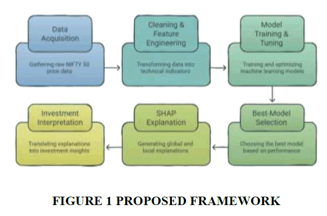
Figure 1 Proposed Framework
Materials and Methods
Dataset
The empirical analysis is carried out using the daily historical data of the NIFTY 50 index which is available with the publicly available data of the National Stock Exchange of India. It contains 6,315 trading days ranging from 3 January 2000 to 26 May 2025, and includes the date along with the open, high, low and close index levels for each trading day. In Section 4.1 descriptive statistics for the price variables are reported. The strong secular upward growth and the notable volatility clustering features are characteristic of an emerging market index, as the closing value of the series increased from about 1,592 in the beginning of the sample to over 25,000 at the end of the sample and peaked above 26,200 during the sample. The working sample is valid until 26 May 2025, which means it covers multiple market regimes, such as the COVID-19 crash in early 2020 and the subsequent lengthy recovery. The evaluation is an out-of-sample test of the framework under regime change which is quite a difficult test as the period of turmoil is in the held-out test set, instead of being a benign in-sample test. Volume-based indicators are not included in the series, and are specified as an extension in Section 10.
Data Cleaning
The raw series were checked and pretreated before the construction of the features. The records were sorted in chronological order, it was checked that the date index was monotonic, there were no non-positive prices, and there were no duplicated dates. There were no trading day gaps (the absence of weekend or holiday rows). Because all subsequent features are constructed exclusively from past information, no forward-looking transformation is applied to the raw prices, and feature standardisation, where required by a learner, is fitted on the training partition only to prevent information leakage.
Feature Engineering
From the cleaned open-high-low-close series we engineer thirty-four features grouped into five families. Return features comprise the daily simple and logarithmic returns and their lags at one, two, three, five and ten days. Trend features comprise simple moving averages over five, ten, twenty and fifty days, the twelve- and twenty-six-day exponential moving averages, the ratios of the close to its twenty- and fifty-day averages, and the MACD line, its signal and its histogram. Momentum and oscillator features comprise the fourteen-day RSI, ten-day momentum, five- and ten-day rate of change, the fourteen-day stochastic %K and its three-day signal %D, the fourteen-day Williams %R, and the twenty-day CCI. Volatility features comprise the percentage-of-price fourteen-day ATR, the rolling standard deviation of returns over five, ten and twenty days, and Bollinger-Band position (%b) and bandwidth. Two intraday-structure features—the high-low range and the close-to-open change, each scaled by price—complete the set. The complete feature inventory is provided in Appendix A. Rows containing the indicator warm-up period and the final undefined target were removed, yielding 6,266 complete observations.
Target Variable
Direction prediction is framed as binary classification. The target for trading day t takes the value 1 (an “UP” day) when the closing level on day t+1 exceeds the closing level on day t, and 0 (a “DOWN” or non-positive day) otherwise. The percentage of positive observations for the modelling sample is 54.0%, and even more so for the held-out test window (55.5%), as the rally since the outbreak of the pandemic has been strong. The appropriate naïve benchmark is thus an always-UP classifier that performs at the current base rate, and all models tested against this base rate instead of against an uninformative benchmark of 50%.
Train-Test Strategy
Financial data are time-ordered, so random shuffling of the data would introduce information about the future into the training data and result in optimistically biased estimates. We thus divide our observations chronologically into 80% (5,012 days, 13 March 2000 to 8 May 2020) for training and 20% (1,254 days, 11 May 2020 to 26 May 2025) for testing, which is never seen during training or tuning. Hyperparameter selection is done with 5-fold time-series cross-validation (TSCV), where each validation fold is strictly following its training fold, which is similar to the walk-forward approach that would be needed when deployedintherealworld.
Machine Learning Models
Five classifiers spanning the linear, single-tree and ensemble families are evaluated. Logistic regression provides a transparent linear benchmark and is fitted on standardised features. A single decision tree, constrained in depth and minimum leaf size, provides an interpretable non-linear benchmark. A random forest (Breiman, 2001) aggregates many decorrelated trees to reduce variance. LightGBM (Ke et al., 2017) and XGBoost (Chen & Guestrin, 2016) are state-of-the-art gradient-boosting implementations that build trees sequentially to minimise a regularised objective; both are widely regarded as the strongest general-purpose learners for structured tabular data, and XGBoost is the focal model of this study.
Hyperparameter Optimisation
The XGBoost hyperparameters were tuned by exhaustive grid search over the number of estimators (200, 400), maximum tree depth (3, 4, 5) and learning rate (0.01, 0.05), with the subsample and column-subsample fractions fixed at 0.8 to regularise the ensemble, using the time-series cross-validation scheme described above and ROC-AUC as the selection criterion. The selected configuration—200 trees of maximum depth four, a learning rate of 0.01, and subsampling of both rows and columns at 0.8—achieved a cross-validated AUC of 0.547 and reflects a deliberately conservative, heavily regularised model appropriate to the low signal-to-noise ratio of the task. The remaining learners were configured with sensible, lightly regularised defaults to ensure a fair comparison.
Performance Metrics
Because directional classes are only mildly imbalanced and the costs of false positives and false negatives are broadly symmetric for an unleveraged directional signal, we report a balanced suite of metrics rather than relying on accuracy alone. Accuracy measures overall correctness; precision and recall characterise performance on the positive (UP) class; the F1-score is their harmonic mean; ROC-AUC measures ranking quality independently of the decision threshold; and the Matthews correlation coefficient (MCC) provides a single, robust summary that is informative even under class imbalance and is zero for a non-informative classifier. The confusion matrix of the focal model is also reported.
Explainability
To interpret the focal XGBoost model we apply SHAP using its exact TreeSHAP algorithm for tree ensembles (Lundberg et al., 2020). SHAP attributes to each feature, for each prediction, an additive contribution measured in the model's log-odds output space, such that the contributions sum to the difference between the prediction and the dataset's expected output. Aggregating the absolute contributions across the test set yields a global importance ranking; examining individual predictions yields local explanations. We report the global beeswarm summary, the global mean-absolute-SHAP bar ranking, a dependence plot for the most influential feature, and a waterfall decomposition of a single trading day's prediction.
Experimental Results
Dataset Statistics
Table 2 reports descriptive statistics for the four price variables over the full sample. The wide gap between the minimum and maximum closing levels, and the standard deviation of comparable magnitude to the mean, reflect the index's strong multi-year growth across the sample window. Figure 2 plots the closing series, making the secular uptrend and the episodes of sharp drawdown—most visibly the 2008 global financial crisis—readily apparent Table 2.
| Table 2. Descriptive Statistics of Nifty 50 Price Variables (2000–2025; 6,315 Trading Days). | ||||
| Statistic | Open | High | Low | Close |
| Count | 6,315 | 6,315 | 6,315 | 6,315 |
| Mean | 7,813.65 | 7,858.81 | 7,758.15 | 7,809.68 |
| Std. dev. | 6,248.40 | 6,270.43 | 6,216.99 | 6,244.65 |
| Minimum | 853 | 877 | 849.95 | 854.2 |
| 25th pct. | 2,851.38 | 2,884.10 | 2,812.65 | 2,850.60 |
| Median | 5,803.05 | 5,857.35 | 5,749.50 | 5,796.90 |
| 75th pct. | 10,786.18 | 10,830.62 | 10,727.78 | 10,781.72 |
| Maximum | 26,248.25 | 26,277.35 | 26,151.40 | 26,216.05 |
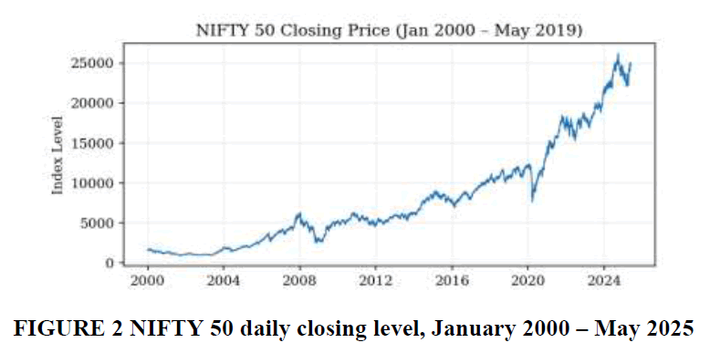
Figure 2 NIFTY 50 daily closing level, January 2000 – May 2025
Correlation Structure of Features
Figure 3 presents the correlation matrix of a representative subset of the engineered indicators. As expected, oscillators that measure related phenomena exhibit strong mutual correlation—the stochastic %K, Williams %R and CCI move together, as do the various volatility measures—whereas the most recent daily return is only weakly correlated with the slower trend and oscillator features. This structure indicates that the feature set, while partially redundant by construction, spans several distinct and complementary information channels, which is precisely the condition under which a regularised ensemble such as XGBoost performs well and under which SHAP attribution is most informative.
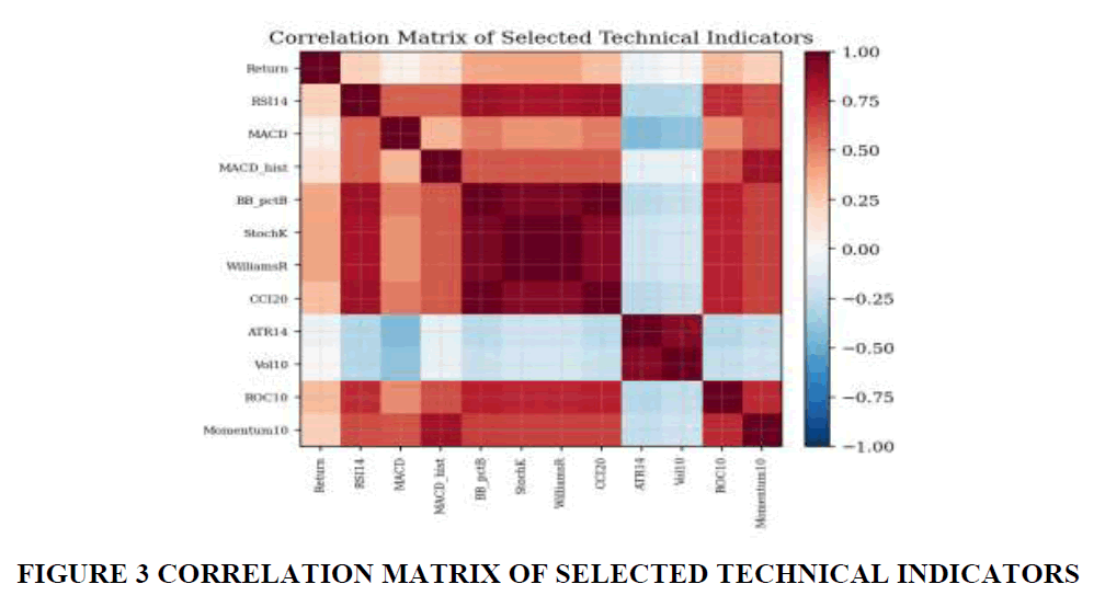
Figure 3 Correlation Matrix of Selected Technical Indicators
Model Performance
Table 3 reports the out-of-sample performance of all five classifiers on the held-out test set, and Figure 4 displays the same results graphically. Three observations stand out, and the first reframes how the remaining two must be read. First, the 2020–2025 test window is strongly bull-biased: 55.5% of test days close higher, so a trivial rule that always predicts UP would itself score 55.5% accuracy. No model exceeds this figure on raw accuracy—the best accuracy, 54.6% from the decision tree, in fact falls just below it—which is a concrete illustration of why headline accuracy is an unreliable and even misleading criterion for directional forecasting in a trending market. Second, on the metrics that actually measure discrimination rather than base-rate matching, the tuned XGBoost model is the strongest learner: it attains the highest ROC-AUC (0.540) and the highest MCC (0.093) of any model, and is the only learner to top both simultaneously. Third, the apparent accuracy advantage of the decision tree is an artefact of class skew rather than skill: its high recall (0.697) reveals a strong tendency to predict the majority UP class, and its MCC of just 0.059—well below XGBoost's—confirms that it captures little genuine signal once the base rate is accounted for. A positive MCC on the other hand indicates the discriminatory ability spread over both UP and DOWN days, unlike XGBoost. These results indicate that XGBoost is the best model to be used as the focal model in the following explanatory analysis.
| Table 3 Out-of-Sample Classification Performance on the Test set not Seen in the Training Process (2020-2025). | ||||||
| Model | Accuracy | Precision | Recall | F1 | ROC-AUC | MCC |
| Logistic Regression | 0.523 | 0.606 | 0.404 | 0.485 | 0.536 | 0.078 |
| Decision Tree | 0.546 | 0.575 | 0.697 | 0.63 | 0.535 | 0.059 |
| Random Forest | 0.518 | 0.622 | 0.336 | 0.437 | 0.539 | 0.089 |
| LightGBM | 0.488 | 0.586 | 0.264 | 0.364 | 0.524 | 0.036 |
| XGBoost | 0.529 | 0.617 | 0.398 | 0.484 | 0.54 | 0.093 |
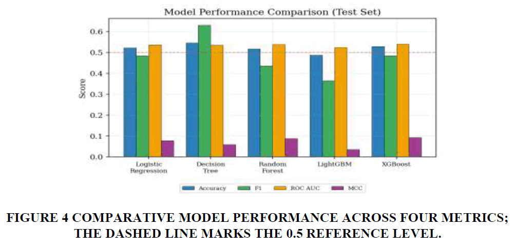
Figure 4 Comparative Model Performance Across Four Metrics; the Dashed Line Marks the 0.5 Reference Level.
The top number in each column is the best number. The highest ROC-AUC and MCC are achieved by XGBoost, while the higher accuracy of the decision tree is due to majority class prediction. This is the test-set baseline accuracy for the "always-UP" majority class, which is 0.555.
Best Model
To explain the focal model, we have to go with the model that performs the best on the discrimination metrics, which in this case is XGBoost. It has a confusion matrix for the testing data set as depicted in Figure 5. The model correctly predicts 277 (recall of 0.398) of the 696 actual UP days and 386 (specificity of 0.692) of the 558 actual DOWN days. Unlike the majority-leaning learners, XGBoost is more likely to predict DOWN than the bullish base rate would have predicted, at the cost of recalling less of the DOWN class, which is how it gets its high MCC score and trumps the base rate prediction, but does so by being more willing to call the minority, DOWN, class, and showing a much better performance on DOWN days.
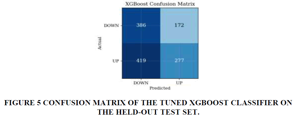
Figure 5 Confusion Matrix of the Tuned Xgboost Classifier on the Held-Out Test Set.
ROC Analysis
The receiver-operating-characteristic curves of the five models are plotted on top of each other in figure 6. It is seen that the curves are almost parallel to the diagonal line of random guessing, with the XGBoost curve on top, followed closely by that of random forest. The small but real separation from the diagonal quantifies a very small bit of ranking ability that the models have: The best of the five learners, XGBoost, has a success rate of about 54.0% when a random UP–DOWN pair is drawn. However, ROC-AUC is bull bias independent of the test window, thus providing a more meaningful comparison than accuracy and together with MCC provides a fairer comparison.
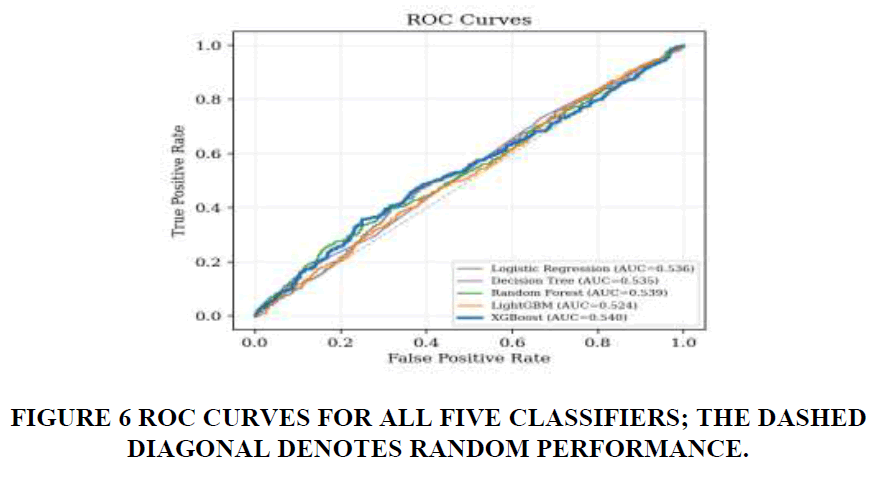
Figure 6 Roc Curves for All Five Classifiers; the Dashed Diagonal Denotes Random Performance.
SHAP Analysis
The prediction constitutes the main analytical task that the paper makes available, having first decided to use XGBoost for prediction. Figure 7 shows the global mean-absolute-SHAP rankings, and Figure 8 the beeswarm summary, which also conveys the direction of the effect of each feature. Table 4 shows the top 10 features according to the mean absolute SHAP value.
| Table 4 Ten Most Influential Features by Mean Absolute Shap Value | |||
| Rank | Feature | Family | Mean |SHAP| |
| 1 | Daily return (t) | Return / momentum | 0.085 |
| 2 | SMA (50-day) | Trend | 0.061 |
| 3 | MACD signal line | Trend | 0.036 |
| 4 | Return lag 5 | Return | 0.028 |
| 5 | MACD line | Trend | 0.026 |
| 6 | RSI (14-day) | Oscillator | 0.025 |
| 7 | Return lag 2 | Return | 0.022 |
| 8 | Volatility (20-day) | Volatility | 0.018 |
| 9 | Stochastic %K | Oscillator | 0.017 |
| 10 | MACD histogram | Trend | 0.016 |
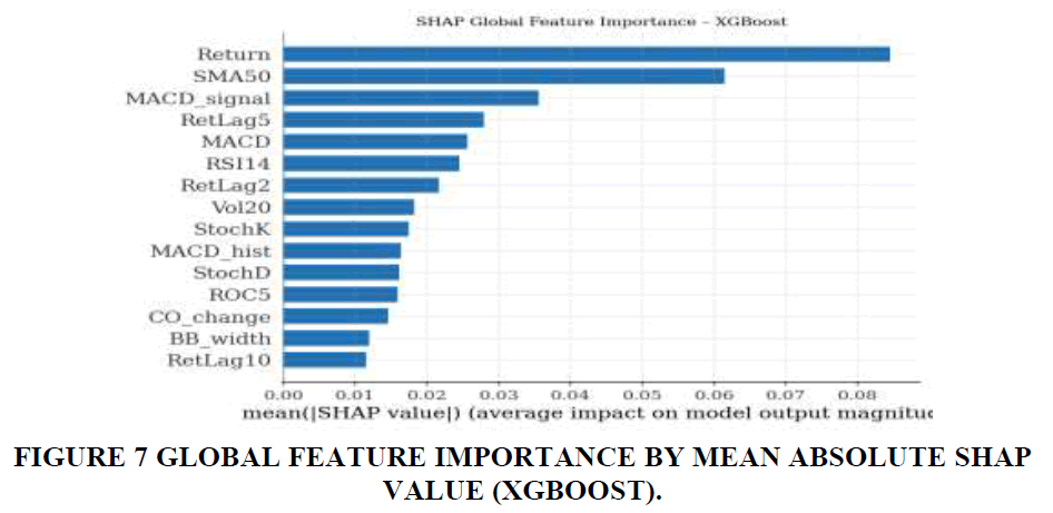
Figure 7 Global Feature Importance by Mean Absolute Shap Value (Xgboost).
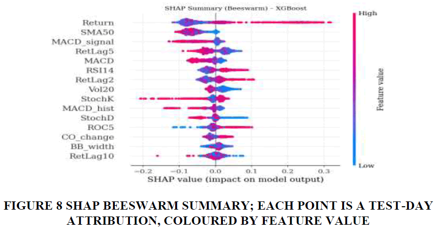
Figure 8 Shap Beeswarm Summary; Each Point is a Test-Day Attribution, Coloured by Feature Value
The attribution makes sense in an economic sense. By far the most important is the most recent daily return, with a mean absolute SHAP value about forty per cent higher than the second most important feature; the beeswarm illustrates that very large daily returns of either sign are the most important feature, reflecting the well-known short-horizon momentum and reversal effects. Analyzing the secondary information channels the model uses, the fifty day SMA is second while the MACD line + signal + histogram are all in the top ten, meaning that trend context in the medium time frame is the strongest one. The fourteen-day RSI together with the stochastic %K over bought/oversold indicator are very strong. The other lagged returns (two-day and five-day) are strong as well highlighting that the model is trading on the short-term autocorrelation of the series. The model also includes the 20-day return volatility indicating the volatility of the risk regime for the condition. Notably, the ranking results from the longer 2000–2025 time period are consistent with the significance of trend and momentum features, rather than the oscillator features that tend to rank better in shorter time periods. In Figure 9, the impact of other features is implicit, yet we examine how the model is dependent on its most important feature, that of the daily return. It is non-linear and non-monotonic: the sign and magnitude of the contribution of the SHAP value changes over the last few years; a linear model would not have been able to capture that behaviour and SHAP would not have made it legible. Figure 10 gives a local explanation for one day in the trading day – it breaks down the model's output into the sum of individual features and explicitly illustrates which signals nudged the model towards an UP or DOWN prediction for that day. This local view is what makes the model an auditable decision aid, as for every forecast, a user can easily find out what are exactly the features that accounted for a forecast.
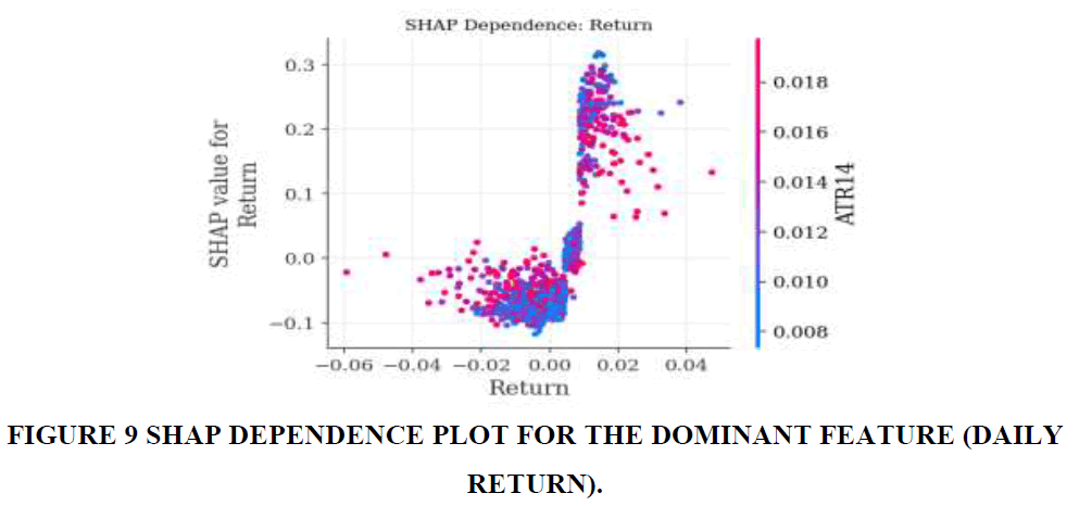
Figure 9 Shap Dependence Plot for the Dominant Feature (Daily Return).
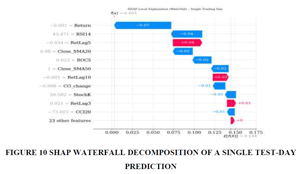
Figure 10 Shap Waterfall Decomposition of a Single Test-Day Prediction
Prediction
Investment Interpretation
A literal financial interpretation is possible for the SHAP results. The pre-eminence of the most recent return and of short-horizon lagged returns suggests that, if the NIFTY 50's next-day direction can be predicted at all, all of the predictability resides in very recent price dynamics, which is more of an empirical signature of short-term momentum and microstructure effects, than of slow fundamental adjustment. The RSI's significance is a testament to the importance that traders give to overbought and oversold levels: the model has been able to learn by itself that the extremes of the RSI are directional signals. The role of the exponential moving averages reinforces the general trend context in the interpretation of a single day's move, and that the twenty-day volatility shows up well reinforces the capacity of the model to discount directionality in times of turbulence. All these attributions combined provide an investor with not only a forecast but a justification put in the common terminology of technical analysis.
Discussion
This study's results need interpretation with regard to two kinds of point of view: predicting and explaining. We are not boastful when it comes to performance and the assessment period is the one that underlines them. The test window for 2020-2025 is heavily skewed towards an upwards trend, and the base rate is so low that it is difficult to prove that any model other than the always-UP model outperforms the trivial one; therefore, we use the non-base-rate driven metrics of ROC-AUC and the Matthews correlation coefficient to evaluate the accuracy of the models. The tuned XGBoost model is the best of the five models and the direction of the NIFTY 50 next day is only slightly predictable based on technical indicators as seen from its AUC score of 0.540 and MCC score of 0.093. We do not consider this to be a "deficiency" of the framework, but rather a “substantively correct result” that is consistent with the weaker form efficient market hypothesis (Fama, 1970) and with the extant empirical literature, where valid out-of-sample accuracy of prediction of the direction of change occurs on average slightly above a chance level for liquid indexes. Near-perfect accuracy on index direction is typically reported in studies which suffer from look-ahead leakage, improper shuffling of time-ordered data or evaluation on in-sample data; our strictly chronological protocol, that includes an entire turbulent regime in the test set prevents those artefacts, and the sober numbers we obtain are, we argue, more trustworthy than inflated alternatives. The robust feature of XGBoost is its regularised sequential boosting of shallow trees, which is able to capture the non-linear interactions between indicators, while mitigating the overfitting problem commonly seen for each individual deep tree or an unregularised ensemble of shallow trees when applied to noisy financial data. It shows that although they are algorithmically similar, boosting implementations can vary a great deal in performance on different data sets, and that a lot of tuning and creativity is required to get the best out of a boosting algorithm for a specific task, rather than opting for a particular library. When it's explained, the contribution is more substantial. The SHAP analysis transforms the black box results of the model in a ranked, signed and economically meaningful representation of which technical signals contribute to the model predictions, at both the population and individual-prediction level. The interpretation is in line with financial intuition, such as recent returns, trend context, momentum oscillators and volatility regime, and this not only confirms the model but also shows the benefits of the explainability layer for diagnostics. In a deployment environment this layer would enable an analyst to see if the model's reasoning over time is stable, whether it's starting to use spurious features or what is the foundation of the model's algorithmic recommendation for a stakeholder or regulator.
Practical Implications
The framework is useful to individual investors as a disciplined and transparent addition to their discretionary technical analysis, and emphasizes the indicators that provide the most direction, not any single "rule of thumb. The explainable signal could form one of a portfolio manager's many inputs into allocation process and SHAP attributions can be used to document and govern model-driven decisions. The local-explanation capability directly meets the model-risk-management and audit needs of financial institutions, unlike opaque models, which cannot give such a rationale per prediction. The ranked feature importances can provide parsimonious feature selection to algorithmic-trading desks, and help mitigate the risk of overfitting and latency by eliminating features with low contribution. The model's volatility feature dependence and the measured moderate accuracy are a deterrent to the overt confidence of the risk manager who is tempted to size positions based on a single-direction signal with moderate strength.
Theoretical Contributions
The study makes a contribution to several literatures. In the machine learning literature it provides a fresh and leak-free comparison of five classifiers to a new emerging-market index and underscores the power of regularised gradient boosting for noisy tabular data. It extends the application of TreeSHAP to the task of forecasting the direction of the next-day index to the explainable-AI literature and shows how the game-theoretic attribution technique can make financial models audit. It gives quantitative, ranked evidence on the relative informativeness of all the common technical indicators for the NIFTY 50 to financial-analytics literature. And to behavioural finance it provides indirect, data-driven support of the salience of short-horizon momentum and overbought/oversold cycles; these cycles are not assumed into the model, but rather inferred from the model's learned attributions.
Conclusion
In this paper, an explainable machine learning system is designed and tested for predicting whether the NIFTY 50 index will move upwards or downwards the following day for the entire time period between 2000 and 2025. Even though the test window, in a strictly chronological evaluation, was held open by the dislocation and recovery from the COVID-19 pandemic, a tuned XGBoost classifier provided the best discrimination of five classifiers based on achieving the highest ROC-AUC (0.540) and the highest MCC (0.093) values. The most recent daily return, the fifty-day simple moving average, the MACD complex, short horizon lagged returns and RSI as well as return volatility were then identified as the strongest factors driving the model's forecasts in a SHAP analysis. The two key findings are: Firstly, the price-based indicators are good at predicting the direction of the NIFTY index for the next day; this is what you would expect from a market that is efficient. And secondly, despite being difficult to explain, AI still provides significant value, improving an opaque ensemble into a transparent, auditable and economically interpretable decision support tool. The value of this clear process is in the open frame, in the honest metric-driven framing, and in the fact that it is not the promise of great predictive ability that the process is valuable, but rather the potential to get it wrong badly in a “trending” market.
Limitations
These findings are subject to a number of limitations which should be considered: The analysis is limited to the NIFTY 50 so the generalisation of the ranking of the indicators to other markets is not tested. The feature set is limited to price-based technical indicators, trading volume (which was not available in the working series) and macro-economic variables like interest rates, exchange rates and inflation are not included, nor is any indicator of news or social-media sentiment. The held-out test window is a good thing because it covers the COVID-19 dislocation and recovery period, but it is very much bull-biased, and that's why we use base-rate-invariant ROC-AUC and MCC for conclusions – a different test window could produce a different ranking of accuracy even if the discrimination was the same. Third, the study concludes on a statistical classification level and not on an economic level net of transaction cost; a positive directional signal on this level would then have to be carefully backtested and evaluated with regard to costs before a conclusion about profitability could be drawn.
Future Research
These limitations chart a clear agenda for future work. The most immediate extension is to incorporate exchange-reported trading volume, enabling volume-based indicators such as on-balance volume and the volume-weighted confirmation of price signals that the present price-only series cannot support. Evaluation could also be made more robust to the choice of test window through walk-forward backtesting across multiple rolling out-of-sample periods, so that performance is not contingent on the bull bias of any single window. Beyond this, the feature space could be enriched with macroeconomic indicators and with textual sentiment derived from financial news using domain-adapted language models such as FinBERT. On the modelling side, sequence architectures—LSTM and gated recurrent networks, temporal convolutional networks and transformer-based models—together with additional gradient-boosting variants such as CatBoost, could be benchmarked within the same explainable protocol, and SHAP could be complemented with counterfactual and attention-based explanations. Finally, the directional signal could be embedded within a reinforcement-learning trading agent and evaluated through cost-aware, real-time and multi-market backtesting to assess its economic, as opposed to merely statistical, value.
References
Adadi, A., & Berrada, M. (2018). Peeking inside the black-box: a survey on explainable artificial intelligence (XAI). IEEE access, 6, 52138-52160.
Indexed at, Google Scholar, Cross Ref
Appel, G. (2005). Technical analysis: power tools for active investors. FT Press.
Ballings, M., Van den Poel, D., Hespeels, N., & Gryp, R. (2015). Evaluating multiple classifiers for stock price direction prediction. Expert systems with Applications, 42(20), 7046-7056.
Barredo, A. A., Del Ser, J., Gil-Lopez, S., Díaz-Rodríguez, N., Bennetot, A., Chatila, R., ... & Benjamins, R. (2020). Explainable Explainable Artificial Intelligence (XAI): Concepts, taxonomies, opportunities and challenges toward responsible AI. Information fusion, 58, 82-115.
Basak, S., Kar, S., Saha, S., Khaidem, L., & Dey, S. R. (2019). Predicting the direction of stock market prices using tree-based classifiers. The north american journal of economics and finance, 47, 552-567.
Indexed at, Google Scholar, Cross Ref
Bollinger, J. (2002). Bollinger on Bollinger bands(p. 0). New York: McGraw-Hill.
Breiman, L. (2001). Random forests. Machine learning, 45(1), 5-32.
Indexed at, Google Scholar, Cross Ref
Bussmann, N., Giudici, P., Marinelli, D., & Papenbrock, J. (2021). Explainable machine learning in credit risk management. Computational Economics, 57(1), 203-216.
Indexed at, Google Scholar, Cross Ref
Bustos, O., & Pomares-Quimbaya, A. (2020). Stock market movement forecast: A systematic review. Expert Systems with Applications, 156, 113464.
Indexed at, Google Scholar, Cross Ref
Carta, S. M., Consoli, S., Piras, L., Podda, A. S., & Recupero, D. R. (2021). Explainable machine learning exploiting news and domain-specific lexicon for stock market forecasting. Ieee Access, 9, 30193-30205.
Indexed at, Google Scholar, Cross Ref
Chen, T., & Guestrin, C. (2016, August). Xgboost: A scalable tree boosting system. In Proceedings of the 22nd acm sigkdd international conference on knowledge discovery and data mining (pp. 785-794).
Indexed at, Google Scholar, Cross Ref
Dhondiyal, A., Chauhan, D., & Munjal, G. (2025). NIFTY 50 stock price prediction using machine learning techniques and technical indicators. In N. Hasteer, S. McLoone, P. Sharma, & R. Nallamalli (Eds.), Adaptive Intelligence (InCITe 2024). Springer.
Fama, E. F. (1970). Efficient capital markets: A review of theory and empirical work. The journal of Finance, 25(2), 383-417.
Indexed at, Google Scholar, Cross Ref
Fathali, Z., Kodia, Z., & Ben Said, L. (2022). Stock market prediction of Nifty 50 index applying machine learning techniques. Applied Artificial Intelligence, 36(1 ), 2111134.
Indexed at, Google Scholar, Cross Ref
Fischer, T., & Krauss, C. (2018). Deep learning with long short-term memory networks for financial market predictions. European journal of operational research, 270(2), 654-669.
Indexed at, Google Scholar, Cross Ref
Goodell, J. W., Kumar, S., Lim, W. M., & Pattnaik, D. (2021). Artificial intelligence and machine learning in finance: Identifying foundations, themes, and research clusters from bibliometric analysis. Journal of behavioral and experimental finance, 32, 100577.
Indexed at, Google Scholar, Cross Ref
Gu, S., Kelly, B., & Xiu, D. (2020). Empirical asset pricing via machine learning. The Review of Financial Studies, 33(5), 2223-2273.
Indexed at, Google Scholar, Cross Ref
Gunning, D., & Aha, D. (2019). DARPA’s explainable artificial intelligence (XAI) program . AI magazine, 40(2), 44-58.
Indexed at, Google Scholar, Cross Ref
Henrique, B. M., Sobreiro, V. A., & Kimura, H. (2019). Literature review: Machine learning techniques applied to financial market prediction. Expert Systems with Applications, 124, 226-251.
Indexed at, Google Scholar, Cross Ref
Hochreiter, S., & Schmidhuber, J. (1997). Long short-term memory. Neural Computation, 9(8), 1735–1780.
Indexed at, Google Scholar, Cross Ref
Jabeur, S. B., Mefteh-Wali, S., & Viviani, J.-L. (2021). Forecasting gold price with the XGBoost algorithm and SHAP interaction values. Annals of Operations Research.
Indexed at, Google Scholar, Cross Ref
Jafar, S. H., Akhtar, S., El-Chaarani, H., Khan, P. A., & Binsaddig, R. (2023). Forecasting of NIFTY 50 index price by using backward elimination with an LSTM model. Journal of Risk and Financial Management, 16(10), 423.
Indexed at, Google Scholar, Cross Ref
Ke, G., Meng, Q., Finley, T., Wang, T., Chen, W., Ma, W., ... & Liu, T. Y. (2017). Lightgbm: A highly efficient gradient boosting decision tree. Advances in neural information processing systems, 30.
Krauss, C., Do, X. A., & Huck, N. (2017). Deep Neural Networks, Gradient-Boosted Trees, and Random Forests for Stock Market Prediction. European Journal of Operational Research, 259(2), 653-664.
Lo, A. W., Mamaysky, H., & Wang, J. (2000). Foundations of technical analysis: Computational algorithms, statistical inference, and empirical implementation. The journal of finance, 55(4), 1705-1765.
Lundberg, S. M., & Lee, S.-I. (2017). A unified approach to interpreting model predictions. In Advances in Neural Information Processing Systems (Vol. 30, pp. 4765–4774). Curran Associates.
Lundberg, S. M., Erion, G., Chen, H., DeGrave, A., Prutkin, J. M., Nair, B., ... & Lee, S. I. (2020). From local explanations to global understanding with explainable AI for trees. Nature machine intelligence, 2(1), 56-67.
Indexed at, Google Scholar, Cross Ref
Mahajan, V., Thakan, S., & Malik, A. (2022). Modeling and forecasting the volatility of NIFTY 50 using GARCH and RNN models. Econ omies, 10(5), 102.
Manjunath, C., Marimuthu, B., & Ghosh, B. (2023). Analysis of Nifty 50 index stock market trends using hybrid machine learning model in quantum finance. International Journal of Electrical and Computer Engineering (IJECE), 13(3), 3549-3560.
Indexed at, Google Scholar, Cross Ref
Mintarya, L. N., Halim, J. N., Angie, C., Achmad, S., & Kurniawan, A. (2023). Machine learning approaches in stock market prediction: A systematic literature review. Procedia Computer Science, 216, 96-102.
Indexed at, Google Scholar, Cross Ref
Murphy, J. J. (1999). Technical analysis of the financial markets: A comprehensive guide to trading methods and applications. Penguin.
Nti, I. K., Adekoya, A. F., & Weyori, B. A. (2020). A systematic review of fundamental and technical analysis of stock market predictions. Artificial Intelligence Review, 53(4), 3007-3057.
Indexed at, Google Scholar, Cross Ref
Patel, J., Shah, S., Thakkar, P., & Kotecha, K. (2015). Predicting stock and stock price index movement using trend deterministic data preparation and machine learning techniques. Expert systems with applications, 42(1), 259-268.
Indexed at, Google Scholar, Cross Ref
Ribeiro, M. T., Singh, S., & Guestrin, C. (2016, August). " Why should i trust you?" Explaining the predictions of any classifier. In Proceedings of the 22nd ACM SIGKDD international conference on knowledge discovery and data mining (pp. 1135-1144).
Indexed at, Google Scholar, Cross Ref
Selvin, S., Vinayakumar, R., Gopalakrishnan, E. A., Menon, V. K., & Soman, K. P. (2017, September). Stock price prediction using LSTM, RNN and CNN-sliding window model. In 2017 international conference on advances in computing, communications and informatics (icacci) (pp. 1643-1647). IEEE.
Indexed at,Google Scholar,Cross Ref
Sezer, O. B., Gudelek, M. U., & Ozbayoglu, A. M. (2020). Financial time series forecasting with deep learning: A systematic literature review: 2005–2019. Applied Soft Computing, 90, 106181.
Indexed at, Google Scholar, Cross Ref
Singh, G. (2022). Machine learning models in stock market prediction. arXiv preprint arXiv:2202.09359.
Indexed at, Google Scholar, Cross Ref
Wallapure Manikrao, K.., Allagi, S., Leong, W. Y., & Laddi, M. (2025). An Explainable AI for Stock Market Prediction: A Machine Learning Approach with XAI and Deep Neural Networks. Journal of Computational and Cognitive Engineering.
Indexed at, Google Scholar, Cross Ref
Weng, B., Ahmed, M. A., & Megahed, F. M. (2017). Stock market one-day ahead movement prediction using disparate data sources. Expert systems with applications, 79, 153-163.
Indexed at,Google Scholar,Cross Ref
Wilder, J. W. (1978). New concepts in technical trading systems. Trend Research.
Appendix A. Feature Inventory and Indicator Definitions
The thirty-four features used in the study are listed below by family. All features are computed using information available up to and including trading day t (Table A1).
| Table A1 Feature Inventory by Family (34 Features in Total). | |
| Family | Features |
| Return / lagged returns | Daily simple return; daily log return; lagged returns at 1, 2, 3, 5 and 10 days. |
| Trend | SMA(5), SMA(10), SMA(20), SMA(50); EMA(12), EMA(26); Close/SMA(20); Close/SMA(50); MACD; MACD signal; MACD histogram. |
| Momentum / oscillator | RSI(14); Momentum(10); ROC(5); ROC(10); Stochastic %K(14); Stochastic %D(3); Williams %R(14); CCI(20). |
| Volatility | ATR(14)/Close; rolling std. of returns over 5, 10 and 20 days; Bollinger %b; Bollinger bandwidth. |
| Intraday structure | High–low range / Close; (Close–Open) / Open. |
Selected indicator formulae
RSI(14) = 100 − 100 / (1 + RS), where RS is the ratio of the 14-day average gain to the 14-day average loss.
MACD = EMA(12) − EMA(26); signal = EMA(9) of MACD; histogram = MACD − signal. Stochastic %K = 100 × (Close − Low14) / (High14 − Low14); %D = 3-day moving average of %K.
Williams %R = −100 × (High14 − Close) / (High14 − Low14).
ATR(14) = 14-day moving average of the true range, expressed as a fraction of the closing price.
Bollinger %b = (Close − lower band) / (upper band − lower band), with bands at the 20-day mean ± two standard deviations.
Appendix B. XGBoost hyperparameter configuration
Information about repeatability and data source (Table B1). All results have been obtained from the daily NIFTY 50 open-high-low-close (6315 trading days, from 3 January 2000 to 26 May 2025). The pipeline—feature engineering, chronological splitting, model training and tuning, and SHAP attribution—is completely deterministic with a fixed random seed and can be reexecuted without changing any parameters with a subsequent extended series or with an additional series of exchange-reported volume that re-calculates each reported figure and table.
| Table B1 Tuned Xgboost Hyperparameters Selected by Grid Search. | |
| Hyperparameter | Selected value |
| Number of estimators (trees) | 200 |
| Maximum tree depth | 4 |
| Learning rate | 0.01 |
| Subsample (row) fraction | 0.8 |
| Column subsample fraction | 0.8 |
| Selection criterion | ROC-AUC (5-fold time-series CV) |
| Cross-validated AUC | 0.547 |
Received: 25-July-2026, Manuscript No. AMSJ-26-17346; Editor assigned: 25-July-2026, PreQC No. AMSJ-26-17346(PQ); Reviewed: 10-Aug-2026, QC No. AMSJ-26-17346; Revised: 17-Aug-2026, Manuscript No. AMSJ-26-17346(R); Published: 25-Aug-2026