Keywords

 

ARIMA, GDP Forecast, ADF Test.

 

Introduction

The current study is focused on studying the analysis of relation between Gross Domestic Product (GDP) growths in the Indian context. The section begins with current scenario of the GDP growth and continues to explain all the sectors covered in the analysis. The dependent and independent variables considered are discussed in detail. GDP is the monetary measure of the market value of all the final goods and services produced in a specific time period, often annually or quarterly. GDP (nominal) per capita does not, however, reflect differences in the living and the inflation rates of the countries; therefore using a basis of GDP per capita at Purchasing Power Parity (PPP) is arguably more useful measuring GDP in a country according to Leo & Ayse (2007) in their study of the Turkish economy. Historically, India has classified and tracked its economy and GDP in three sectors: agriculture, industry, and services. Agriculture includes crops, horticulture, milk and animal husbandry, aquaculture, fishing, sericulture, aviculture, forestry, and related activities. Industry includes various manufacturing sub-sectors. India's definition of services sector includes its construction, retail, software, Information Technology (IT), communications, hospitality, infrastructure operations, education, healthcare, banking and insurance, and various economic activities according to the Economic Survey of India (2018).

Literature Review

Singh, et al. (2010) studied the relationship between credit Growth in India in the last few decades, have used unit root test, and Augmented Dickey Fuller (ADF) test, studied the relationship between credit growth and GDP growth in different sectors of the economy, in order to ascertain long term co- integration relationship between Credit and GDP. Hussin & Saidin (2012) examined the contribution of economic sectors to growth in India. This study used secondary data and ascertained the contribution of 3 economic sectors including agriculture, manufacturing and service sectors and studied the contribution to the economic growth in India. (Jain, et al., 2009) investigated the impact of various macro-economic factors on GDP components. This study used secondary data from Securities and Exchange Board of India (SEBI) and the Planning Commission Report of 2013. The study found significant effect of FDI, net FII equity and import on GDP components. The percentage share of the agriculture, in the total GDP has declined. On the contrary, share of the services in the total GDP had increased, the study found. Prochniak (2011) analyzed the impact of the development and stability or the financial sector on economic growth. This study shows the estimation of the regression equations of where the GDP growth rate is regressed against a number of factors including a variable representing financial sector and several variables. The paper analyzed the theoretical and aspherical relationship between the financial system and economic growth attempting to answer the question on what level of financial system development positively influences GDP dynamics.

Motivation for the Current Research

The authors were curious to investigate the nature of the GDP function in India. Specifically, the question was whether the GDP could be broken into the components of Trend (long term), Seasonal (repetitive pattern after “N” quarters). The authors also wanted to verify whether the use of a time-series tool such as Auto Regressive Integrated Moving Average (ARIMA) would yield statistically significant coefficients. The contribution to the literature is that of isolation of the number of Lag periods as well as the ARIMA Coefficients, which can be useful in prediction of GDP in future years.

Problem Statement

The aim of this research is to identify the three components of GDP (Trend, Seasonal and Random) and arrive at a predictive formulation for the forecast of future values of the GDP with the help of Statistical Tools such as the ADF, Partial Auto Correlation Function (PACF) Diagram and finally the ARIMA. All these tools can be found in the python programming environment with the help of packaged libraries such as statsmodels, scipy, numpy and matplotlib.

Problem Solving Methodology

First, the raw GDP data for India was obtained from the Quandl Database. This data was then imported into statistical package within python to decompose into the three components of Trend, Seasonal and Random Components. Next, an Augmented Dickey Fuller (ADF) Test was run on the GDP Data in order to find the number of Lags. In order to corroborate the finding from the ADF Test a PACF Diagram was constructed in order to finalize the number of Lags to be used.

Finally, the ARIMA tool was used in order to predict the coefficients with the number of Lags suggested in the PACF Diagram. The ARIMA coefficients were tested for Statistical significance by observing the p-values. Finally the Forecasted GDP was arrived at by using the ARIMA forecast so developed and the Forecasted GDP was plotted against the Actual GDP for the time period being used in the study.

Results and Discussion

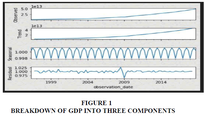
Figure 1 shows that the GDP can be broken into three components. The long term Trend is almost linear and can be forecasted. The Seasonal Trend is repetitive and fluctuates in a manner such that it repeats every 4 quarters (1 Year), leading to an assumption that the number of lags could possibly be 4 (quarters). Finally, it is evident that the Residual component is Random and cannot be forecasted.

Table 1 shows that there is time dependency of GDP across quarters, since the Test Statistic and the Result of the ADF Test indicate that the Data are not stationary and indeed have some time- series effect. Had there been no time-series effect the data would have been stationary. The p- values and ADF Statistic above are obtained for 2 and 4 Lags, respectively.

Table 1 Augmented Dickey Fuller Test (ADF) for Absolute Value of GDP
Number of Lags used (number of Observations)	ADF Test Statistic	p-value	Result
2 (87)	4.45	1.0	Data Not Stationary
4 (57)	-7.13	0.99	Data Not Stationary

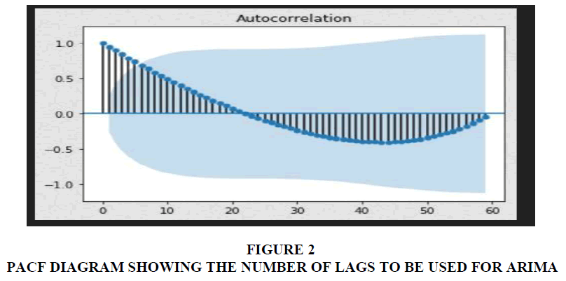
When the Raw GDP Data are plotted for Auto Correlation with the PACF diagram, the number of lags (the lines outside the light blue zone) when counted are 6 in number, implying that the number of lags to be used is in the range of 4 to 6. In conjunction with the inference drawn from Figure 1, where the seasonal effect appears to indicate that the number of lags to be used=4.

Therefore, the ARIMA is constructed using 4 lags, and the results from the ARIMA are tabulated in Table 2 and Figure 2.

Table 2 Augmented Dickey Fuller Test (ADF) for Absolute Value of GDP
Dep. Variables :	GDP	No. of observation	60
Model	SARIMAX (0,4,0)x(1,1,1,4)	Log likelihood	-1546.412
Date	Wed,19 june 2019	AIC	3098.823
Time	12:42:37	BIC	3105.106
Sample	01-01-2019	HQIC	3101.281
Covaiance type	opg

	Co efficient	Std err	Z	p>(z)	0.025	0.975
ar.S.L4	0.5478	0.195	2.807	0.005	0.165	0.930
Ma.S.L4	-0.9015	0.199	-4.521	0.000	-1.295	-0.511
Sigma2	4.464e+24	nan	nan	nan	Nan	nan

Ljung -Box (Q)	108.77	Jarque bera (JB)	0.81
Prob (Q)	0.00	prob (JB)	0.67
Heteroscedasticity (H)	4.01	Skew	-0.20
Prob (H) ( two sided)	0.01	kurtosis	3.45

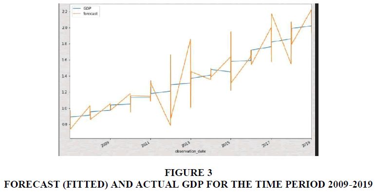
Based on the ARIMA results, for 4 lags we get statistically significant results and the pvalue for the coefficients is 0.005 for the AR (Auto-regressive) component and MA for the Moving Average components. With this, the forecast for GDP is constructed and shown in Figure 3 below.

From Figure 3, it is evident that the forecasted model using the ARIMA coefficients is functional and is producing results which are close to the Actual GDP. This shows that the Assumptions of the Lag are justified and also that the ARIMA coefficients are accurate. A similar study using ARIMA to predict India GDP for a decade was done by Changle, et al. (2016) who found a fit with the ARIMA model. This research has focused on derivation of the ARIMA coefficients for the India GDP as a time-series model. It can be concluded that the number of lags which is useful for accurate model building is 4 quarters. It can also be concluded that the AR component of the ARIMA has a coefficient of 0.5478 and the MA component of the ARIMA coefficient has a value of -0.9015.

References

1. Hussin, F., & Saidin, N. (2012). Economic growth in ASEAN?4 countries: A panel data analysis. International Journal of Economics and Finance, 4(9).
2. Jain, D., Nair, S.K., & Jain, V. (2015). Factors affecting GDP (Manufacturing, Services, Industry): An Indian perspective. Annual Research Journal of Symbiosis Centre for Management Studies Pune, 3, 38-56.
3. Leo, N.K., & Ayse, N. (2007). Purchasing power parity approach in Turkey after 1980, Marmara University I.I.B.F. Journal, 23(2), 9-43.
4. Prochniak, M., (2011). Determinants of economic growth in Central and Eastern Europe: the global crisis perspective. Post-Communist Economies, 23(4), 449-468.
5. Singh, C., Pemmaraju, S., & Das, R., (2016). Economic growth and banking credit in India. IIM Bangalore Research Paper No. 531. Available at SSRN: https://ssrn.com/abstract=2882398 or http://dx.doi.org/10.2139/ssrn.2882398
6. Changle, R., Matharu, S., Choudhary, A., & Malhotra, G. (2016). India’s GDP-The Next Decade: A Forecast Using ARIMA Model, available online at pioneerjournal.in/conferences, accessed on 18th September 2019.
7. Economic Survey (2017-2018). Volume 2, Services Sector Chapter 9 available online at http://mofapp.nic.in:8080. accessed on 18th September 2019.