Research Article: 2022 Vol: 23 Issue: 1S
Bayesian Vector Autoregressive and Co-Integration Modeling of Macroeconomic Variables
Fentahun Yeshaneh Nigatie, ODA Bultu University
Sefinew Gebeyehu Kebede, Debark University
Citation Information: Nigatie, F.Y., & Kebede, S.G. (2022). Bayesian vector autoregressive and co-integration modeling of macroeconomic variables. Journal of Economics and Economic Education Research, 23(S1), 1-15.
Abstract
This study aims to investigate the relationship among Macroeconomic variables annually collected data from the national bank of Ethiopia, Central Statistical Agency, and World Bank website from a period of 1980-2018 by using BVAR approach. Based on a study, granger causality shows unidirectional the change in consumer price index (inflation) and unemployment leads to changes to real GDP growth. Similarly, unidirectional from UR to CPI shows that unemployment leads to a change in inflation. Empirical results of impulse response function analysis show that shock to RGDP leads to a negative response from unemployment which dies out after four years horizons, while the shock to RGDP from inflation of goods and services produces continuous positive responses. BVAR is the appropriate model used to forecast and estimate large macroeconomic variables by reducing the gap between actual and predicted values. The policy implication of this finding is that country should control unemployment and interest by creating different small enterprise led industrialization strategy and expands the investments for Youth.
Keywords
Vector Autoregressive, Co Integration Modeling, Macroeconomic Variables, VAR.
JEL Classifications
C01, C11, C22.
Introduction
Macroeconomics is an analysis of economic structure, performance, and the government’s policies in affecting its economic conditions of a given country. Economists are interested to know the factors that contribute towards the economic growth of a country because if the economy progresses, it will provide more job opportunities, goods, and services and eventually raise the living standard of people (Dougals, 2017).
Macroeconomic policy determination requires a compensating of risks and uncertainties. Governments use macroeconomic forecasts in order to evaluate and develop economic policy. Gross Domestic Product (GDP), demonstration of wealth, is a measure of output which ensures macroeconomic management, so GDP forecasts are capital importance. The Real Gross Domestic Product (RGDP) describes the values of final goods and services which were produced within the boundaries of countries during the time period of more than one year. When people are actively seeking for a job and they are unable to found a work is known as unemployment. According to International Labor Organization definition unemployment as people looking for a last four week, but they cannot found a work (Serneels, 2004).
Unemployment is the macroeconomic problem that affects people most directly and harshly by reduced in the living standard and psychological distress for most people. Unemployment is a frequent topic of political debate and that most politicians often claim that their proposed policies would help to reduce it by creating jobs (Ali, 2014; Dickey & Fuller, 1981).
Granger Causality Results shows that unemployment and inflation does not granger cause wage rate. This result indicates one-way causation flowing from unemployment to wage rate not inflation to wage rate. Unemployment has a positive effect on the wage rate but on the other hand, inflation cannot effect on wage rate (Malam et al., 2013).
Inflation, which raises the price level in a country, creates financial problems in raising the prices of commodities, services, and other factors. Increase in the general price level of goods and services over a specific period in an economy is known as inflation (Rashid & Kemal, 1997). When the price level rises, each unit of currency buys fewer goods and services; consequently, inflation is also erosion in the purchasing power of money, a loss of real value in the internal medium of exchange and unit of account in the economy.
The GDP describes the values of final goods and services which were produced within the boundaries of countries during the period of one year. It has a very important effect on economic growth (Fama, 1975).
BVAR models were used to analyze the capability of forecasting the Ethiopian economy with the key macroeconomic variables relative to alternative methods of forecasting. This study focused on Bayesian Vector Auto-Regression (BVAR) models, annually data over the past thirty nine-years. The previous study conducted more on the relationship between inflation, unemployment, and economic growth by using Vector Auto-Regression (VAR) and multivariate time series approaches. But, this study was conducted on the relationship among macroeconomic variables and economic growth in Ethiopia using BVAR and co-integration model. Specifically, the study was conducted to examine the short-run and long-run relationship between the key macroeconomic variables and investigate the direction of causality between macroeconomic variables in Ethiopia. In addition, this study forecasts the key macroeconomic variables using the BVAR model.
Literature Review
Macroeconomic variables such as interest rate, inflation rate, unemployment rate, and real GDP on the multivariate BVAR models have been found to produce the most accurate short-term and long-term relative to the univariate and unrestricted Classical VAR models. Moreover, the BVAR models are also capable of correctly predicting the direction of change of the macroeconomic variables (Koop & Korobilis, 2013).
Interest is essentially a charge to the borrower for the use of an asset. Interest rate is the amount a lender charges a borrower and is a percentage of the principal the amount loaned. The interest rate is expected to have either a positive or negative impact on economic growth. Thus decreasing the interest rate due to expansionary monetary policy may stimulate the economy because of increased economic activities. Interest rates play a crucial role in the efficient allocation of resources aimed at facilitating the growth and development of an economy.
Analyzing the tradeoff among inflation, interest, and unemployment rate of Pakistan, (Mahmood, 2013) find interest and unemployment rates have a negative impact on the rate of inflation. The study finds that an increase in inflation also raises the level of interest rate. The unemployment rate is impacting the interest rate and inflation rate. However, a significant tradeoff is exists among these variables in the long run.
Analyzing inflation and interest rate for Jordan throughout 1990 to 2012, Granger causality test results show bidirectional causality between inflation and unemployment, economic growth, and budget deficit. The results show a weak positive relationship between inflation and interest rate, due to the unfavorable economic conditions of Jordan over the estimated period Jaradat & AI-Hhosban (2014).
Based on the study conducted on the relationship between unemployment, inflation, and economic growth in Nigeria using the OLS regression method, their results confirmed that interest rate and total public expenditure bares significant impact on economic growth in the long run whereas, on the contrary, inflation and unemployment have inverse effects on growth. The study concludes with a confirmative note on the existence of a causal linkage between inflation, unemployment, and economic growth (Yelwa et al., 2015).
Empirical results of impulse response function analysis show that shock to RGDP leads to a negative response from unemployment which dies out after four years horizons, while the shock to RGDP from inflation of goods and services produces continuous positive responses. There is a long run relationship based on the Johansson Co-integration test and short- run relationship based on VECM among economic growth indicator variables and the vector error correction model(VECM) is appropriate than VAR model infers that the current real economic growth of Ethiopia. Granger causality shows unidirectional the change in consumer price index (inflation) and unemployment leads to changes to real GDP growth and unidirectional from unemployment rate (UR) to consumer price index (CPI) which shows that unemployment leads to change of inflation. The forecast error variance decomposing (FEVDs) tests results indicate that most of the variance in each variable is attributable or explained by own shocks the first and second horizons (Endalew, 2017).
Data and Methodology
Source of data: The source of data was from sets of time series annual recorded data on the key macroeconomic variables from the National Bank of Ethiopia, Central Statistical Agency (CSA), and the World Bank (WB) website statistical bulletin within a period of 1980 to 2018.
Methodology
This study was concerned with modeling multivariate time series data. For many time series arising in practice, a more effective analysis may be obtained by considering individual series as components of a vector time series and analyzing the series jointly. We assume k time series variables, denoted as  are of interest, and we let
 the time series vectors at time t for
  multivariate process arise when several related time series are observed simultaneously over time (Brewin, 2010). Time series is said to be stationary if its mean and variance are constant over time and the value of the covariance between the two periods depends only on the distance or gap or lag between the two time periods and not the actual time at which the covariance is computed. In the time series literature, such a stochastic process is a weakly stationary or covariance stationary (Gujarati & Porter, 2003). Stationary is defined as a fundamental property underlying almost all time series statistical models. Time series is said to be stationary if its mean and variance are constant over time and the value of the covariance between the two periods depends only on the distance or gap or lag between the two time periods and not the actual time at which the covariance is computed. In the time series literature, such a stochastic process
  is a weakly stationary or covariance stationary (Gujarati & Porter, 2003; Shahid, 2014). The stochastic process is said to be stationary if:
 (1)
(1)
 (2)
(2)
From equation [1] all  have the same finite mean vector
  and [2] requires that the auto covariance of the process do not depend on “t” but, just on the time period “j” the two vectors and
  is apart. Therefore, a process is known as stationary if its first and second moments are time invariant. Frequently, if the two methods are not fulfilled then differencing may be needed to achieve stationarity. To test for stationarity of a series several procedures have been developed. The most popular ones are time plot and Unit root test such as ADF and PP test. BVAR models were used to present a solution to the excessive number of parameters to estimate in VAR models by imposing some general restrictions through prior probability distribution functions (Todd, 1990). The data were compiled by using STATA 14 and Eviews 8 statistical software.
Data Estimation and Interpretation
Presentation of result: The study was based on the yearly time series data observed from 1980 to 2018. The total number of observations was 39. In this study, the results of the BVAR model specifications were used for forecasting macroeconomic variables. In Table 1 result, economic growth increased from its minimum value of 101802.6 in 1980 to its maximum value of 1719491.0 in 2018 measured as real GDP. The inflation of goods and services as a percent of GDP increased from their minimum values of 12.924 in 1980 to their maximum value of 252.1015 in 2018. The interest rate (IR) is increased from its minimum value of 0.03 in 1980 to its maximum value of 0.109 in 2018. Similarly, the Unemployment rate is increased from its minimum value of 2.098 in 1980 to its maximum value of 8.71 in 1999.
| Table 1 Descriptive Statistics of the Series: 1980 to 2018 | ||||
| Variable | CPI | IR | RGDP | UR |
| Observation | 39 | 39 | 39 | 39 |
| Mean | 69.34411 | 0.058280 | 340268.9 | 4.695 |
| Median | 34.71918 | 0.059167 | 178512.7 | 5.0930 |
| Maximum | 252.1015 | 0.109000 | 1719491. | 8.7100 |
| Minimum | 12.92441 | 0.030000 | 101802.6 | 2.098 |
| Std.Dev | 72.88473 | 0.021659 | 397818.7 | 1.739 |
| Skwness | 1.428644 | 0.997387 | 2.480018 | 0.4026 |
| Kurtosis | 3.6019 | 3.592582 | 8.292900 | 2.4397 |
| Jargue-Bera | 13.856(0.00098) | 7.0367(0.029648) | 85.50(0.000) | 1.564(0.457) |
Stationary Test
The time series under consideration should be checked for stationary before one can attempt to fit a suitable model. This means that, variables have to be tested for the presence of unit root(s) there by the order of integration of each series is determined. Figure 1 suggests that the series of the endogenous variables display a non-stationary behavior.

Figure 1 Time Series Plot of RGDP, CPI, IR, and UR (at Level)
The Figure 2 result shows that each of the macroeconomic variables individually has stationary time series behavior after first differencing. It indicated that the first differencing is adequate to fit the macroeconomic time series model.

Figure 2 Time Series Plot of LNRGDP, LNCPI, LNIR, and LNUR (After First Deference)
Table 2 indicates that the null hypothesis that the series in levels contain unit root could be not rejected for all the series. Since the null hypothesis cannot be rejected, to determine the order of integration of the non-stationary time series, the same tests were applied to its first difference.
| Table 2 Unit Root Test Results (Original Series) | |||||
| Series | Level with intercept | ||||
| Test statistic | prob** | ||||
| ADF | PP | ADF | PP | Conclusion | |
| CPI | -3.422248 | 0.0656 | 0.571376 | 0.9992 | Non stationary |
| IR | -1.811528 | 0.6794 | 0.47000 | 0.5911 | Non stationary |
| RGDP | 2.93247 | 1.0000 | 1.000 | 1.0000 | non stationary |
| UR | -2.0098 | 0.6429 | 0.28150 | 0.7882 | Non stationary |
The order of integration is the number of unit roots that should be contained in the series to be stationary. The result indicates that we reject the null hypothesis for the first differenced series with intercept and trend at the 5% level of significance for all macroeconomic variables. Since CPI, IR, RGDP, and UR are stationary. Thus, we can say the series are all integrated of order one (I (1)).
And also with the same procedure, there is a stationary at the first difference with intercept and trend also, the first difference without intercept and trend Table 3.
| Table 3 Unit Root Test Results (the First Difference with Intercept) | |||||
| Series | First difference with intercept | ||||
| Test statistic | Prob** | ||||
| ADF | PP | ADF | PP | Conclusion | |
| CPI | -4.587028 | -4.602047 | 0.0007 | 0.0007 | Stationary |
| IR | -5.744362 | -5.754452 | 0.0003 | 0.0003 | Stationary |
| RGDP | -5.14882 | -5.146134 | 0.0001 | 0.0001 | Stationary |
| UR | -5.578124 | -5.754351 | 0.0007 | 0.0007 | Stationary |
BVAR Model Specification
Correlation Matrix: Table 4 shows that there exists high positive correlation between RGDP and CPI, in the same manner; RGDP and UR have weak positive correlation. RGDP and IR have weak negative correlations. CPI and IR have weak negative correlations. CPI and UR have a strong positive correlation. UR and IR have a weak negative correlation. Here the negative correlations indicates that one variable value increases the other variable value is decreased and the positive correlation shows that simultaneously as one variable increases the other variable also increase in the same manner that has correlated variables.
| Table 4 Correlation Matrix of the Variables | ||||
| LNRGDP | LNCPI | LNIR | LNUR | |
| LNRGDP | 1.000000 | 0.959483 | -0.364411 | 0.472969 |
| LNCPI | 0.959483 | 1.000000 | -0.310080 | 0.533601 |
| LNIR | -0.364411 | -0.310080 | 1.000000 | -0.278199 |
| LNUR | 0.472969 | 0.533601 | -0.278199 | 1.000000 |
Estimating of Order BVAR Model
Table 5 results, for determining the most appropriate lag length for the VAR model the Akaike information criterion (AIC), Schwarz Bayesian information criterion (SBIC), and Hannan-Quin information criteria (HQIC) were used. The AIC, SBIC, and HQIC tests suggest appropriate lag length for the VAR model is one (1). That is, the best fitting model is the minimum value of AIC or SBIC, or HQIC.
| Table 5 Estimating of Lag Order | ||||
| Lag | Log L | AIC | SC | HQ |
| 0 | 56.7994 | -2.93330 | -2.7576 | -2.872 |
| 1 | 236.77 | -12.0428* | -11.1630* | -11.7357* |
| 2 | 243.26 | -11.51481 | -9.931292 | -10.96212 |
| 3 | 267.1846 | -11.95470 | -9.667392 | -11.15637 |
The study showed that BVAR (1) is selected by the criterion and BVAR (1) is the best since it has the minimum AIC, SBIC, and HQIC (Table 5). Based the study result, we can use the BVAR (1) model for prediction and forecasting purposes shown in equations [3-5].
Therefore, the BVAR (1) model to be estimated at lag 1 and p=4 are:
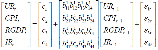 [3]
[3]
Bayesian VAR Model Estimates
Based on n Table 6, the data is incorporated into the posterior distribution only through sufficient statistics, formulas for updating the prior into the posterior coefficients of parameter of a prior is known as hyper-parameters. Where Mu is the prior mean, L1 is lambda1 of over tightness of the variance, L2 is the lambda 2 of relative-variable weight and L3 is Lag decay (Litterman, 1986).
| Table 6 Bayesian Var Estimates | ||||
| Prior type: Litterman/Minnesota Initial residual covariance: Univariate AR Hyper-parameters: Mu: 0, L1: 0.1, L2: 0.99, L3: 1 Standard errors in ( ) & t-statistics in [ ] |
||||
| LNRGDP | LNCPI | LNIR | LNUR | |
| LNRGDP(-1) | 0.562985 | 0.232929 | -0.183576 | -0.063588 |
| (0.06339) | (0.05398) | (0.09799) | (0.07102) | |
| [ 8.88179] | [ 4.31490] | [-1.87347] | [-0.89537] | |
| LNCPI(-1) | 0.399677 | 0.800717 | 0.130730 | 0.122195 |
| (0.05312) | (0.04530) | (0.08218) | (0.05958) | |
| [ 7.52393] | [ 17.6775] | [ 1.59086] | [ 2.05110] | |
| LNIR(-1) | -0.067819 | -0.051894 | 0.474473 | 0.060806 |
| (0.04217) | (0.03599) | (0.06572) | (0.04743) | |
| [-1.60829] | [-1.44171] | [ 7.21955] | [ 1.28193] | |
| LNUR(-1) | -0.039861 | 0.022873 | -0.197651 | 0.635469 |
| (0.04775) | (0.04077) | (0.07410) | (0.05387) | |
| [-0.83481] | [ 0.56107] | [-2.66718] | [ 11.7958] | |
| C | 1.656659 | -0.966580 | 0.229910 | 0.461125 |
| (0.25957) | (0.22106) | (0.40128) | (0.29088) | |
| [ 6.38239] | [-4.37246] | [ 0.57294] | [ 1.58527] | |
| R-squared | 0.976747 | 0.987650 | 0.718135 | 0.851746 |
| Adj. R-squared | 0.973928 | 0.986153 | 0.683969 | 0.833776 |
| Sum sq. resids | 0.099998 | 0.071676 | 0.259177 | 0.143807 |
| S.E. equation | 0.055048 | 0.046605 | 0.088622 | 0.066014 |
| F-statistic | 346.5397 | 659.7521 | 21.01930 | 47.39776 |
| Mean dependent | 5.374442 | 1.659838 | -1.262917 | 0.649583 |
| S.D. dependent | 0.340921 | 0.396048 | 0.157644 | 0.161915 |
BVAR Model - Substituted Coefficients
LNRGDP = 0.561*LNRGDP(-1)+0.3997*LNCPI(-1)-0.0679*LNIR(-1)-0.0399*LNUR(-1)+1.6567 [4]
LNCPI = 0.231*LNRGDP(-1)+0.8007*LNCPI(-1)-0.519*LNIR(-1)-0.0229*LNUR(-1)+0.96658044975 [5]
LNIR = 0.1836*LNRGDP(-1)+0.1307*LNCPI(-1)-0.4745*LNIR(-1)-0.1977*LNUR(-1)+0.2299 [6]
LNUR = -0.0636*LNRGDP(-1)+0.1222*LNCPI(-1)-0.0608*LNIR(-1)-0.6355*LNUR(-1)+0.4611 [7]
The overall statistically significant positive coefficient of  and
and  imply that the effect of a unit increase in first per-determined value of Real GDP growth and first perdetermined value of inflation (consumer price index) while keeping other factors constant then results of current Real GDP growth is increased by 56.1% and 39.37% respectively. Based on the result of the fitted BVAR model, in addition to its own and one year’s lag effect of real economic growth, a significant impact of inflation of goods and services, interest rate and unemployment rate in the past one year’s lag on current economic growth is detected in the study period. This shows that real economic growth of Ethiopia has a significant dynamic relationship among consumer price index (inflation), interest rate and Unemployment rate during the study period. The Adjusted R-square value for this model is 0.97, indicating that 97% of the variation in the future Real GDP growth observation is explained.
Co-Integration Analysis
The procedure for co-integration involves determination of the existence of the long run equilibrium relationship, but does not explain the direction of the causality of the macroeconomic variables. If the variables are no co-integrated, then long run equilibrium relationship does not exist hence only short run relationship can be existing (Johansen, 1991). Since the variables are integrated of order one, we proceed to test for Co-integration. Johansen (1995) Co-integration test is applied at the predetermined lag 1. In these tests, Maximum Eigen value statistic or Trace statistic is compared to critical values. The maximum Eigenvalue and trace tests precede sequentially from the first hypothesis no co-integration to an increasing number of co-integration vectors. Based on Johansen Co-integration tests natural logarithm of RGDP, CPI, IR, and UR are reported Table 7 by using the assumption linear deterministic trend. Based on this output the trace statistic indicates that at least one Co-integration vector (r ≥ 1) exists in the system at 95 percent confidence level 24.36267 < 29.79707 and its p-value (0.1855) is greater than 5% level of significance. In order to cross check for identifying the specific number of Co-integration vectors, by using the maximal Eigenvalue statistic is further employed. This statistic confirms the existence of only one co-integration relationship at 95 percent confidence level 18.8809 < 20.13162 and its p-value (0.1777) is greater than at 5% percent critical value. Based on Johansen Co-integration test of co-integration the trace statistic and maximal Eigenvalue statistic the macroeconomic variables are integrated at one I (1).
| Table 7 Johansen Co-Integration Test Results (by Assumption: Liner Deterministic Trend) | ||||||||||
| Hypothesized Numberof Co-integration vector |
Eigen value | Trace Test | Maximum Eigenvalue Test | |||||||
| Test statistics | 5% critical value | Prob** | Test statistics | 5% critical value | Prob** | |||||
| None* | 0.487430 | 49.09040 | 47.85613 | 0.0381 | 28.58434 | 25.72774 | 0.0113 | |||
| At most 1 | 0.366338 | 24.36267 | 29.29707 | 0.1855 | 18.88087 | 20.13162 | 0.1777 | |||
| Normalized co-integration coefficients(standardized error in parenthesis) 1 co-integrating Equation(s) | ||||||||||
| RGDP | CPI | IR | UR | |||||||
| 1.000000 | -1.223899 | 1.453936 | 0.523220 | |||||||
| (0.15544) | (0.30933) | 0.30916) | ||||||||
The Co-integration vector is given by β=(1,-1.223899,1.453936, and 0.523220). The values correspond to the co-integrating coefficients of natural logarithm RGDP (normalized to one), CPI, IR and UR respectively. Thus, the vector above can be expressed as follows:
 [8]
[8]
Vector Error Correction Model (Vecm) Estimation
Based on the co-integrating vector equation [6] the current RGDP of economic growth is increased by 1.2239 as a unit increasing of the current inflation of goods and service or Consumer Price Index in Ethiopia. Similarly for a unit increase of interest rate, the current RGDP of economic growth of Ethiopia is decreased by 1.4540. For a unit of increase of unemployment rate, the current RGDP of Ethiopia is decreased by 0.5232.
Model for RGDP Growth
 [9]
[9]
Model for CPI
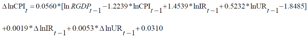 [10]
[10]
Model for IR
 [11]
[11]
Model for UR
 [12]
[12]
 Stands for first difference (D), the value in the bracket are the error correction term and the coefficients of error correction term are called adjustment coefficients.
Based on VECM of the Real GDP growth model under equation [7-12], the coefficient of Co-integrated vector (-0.133) is negative and significant by using OLS estimation method. This shows that the speeds of adjustment towards long run were at equilibrium causality. Under this model there is long run causality from the three independent variables CPI, IR and UR to RGDP. It implies that CPI, IR and UR have influence on the dependent variable of RGDP growth in long run causality. To find the short run causality among variables by using Wald test statistic to the coefficient of CPI. In this model Wald statistic of the coefficient of CPI indicates that there is positive short run causality running from CPI to GDP since p-value is less than 5% level of significance. This result is agreed to (Eden, 2012; Jaradat, 2013) findings. There is negative short run relation causality running from IR to RGDP, since p-value is less than 5% level of significance. Similarly there is negatively short run causality running from UR to RGDP based on OLS estimation of the model and Wald test of the coefficient of UR in the RGDP growth model and the result is coincide with (Kaushik et al., 2015; Giannone et al., 2014) findings. The study result indicates that there is negatively short run causality between Unemployment rate and Consumer Price Index (inflation) in Ethiopia which is agreed with to (Umaru & Zubairu, 2012) findings.
Structural BVAR Analysis
Granger causality test: Granger causality test is considered a useful technique for determining whether one time series is good for forecasting the other. The concept of granger causality test is explored when the coefficients of the lagged of the other variables is not zero (Engle & Granger, 1987).
The result showed Table 8 that CPI granger causes RGDP, while the converse is not true at 5% level of significance. This indicates that the change CPI precedes the change in RGDP, and that the last information on CPI provides important information to forecast future value of RGDP. In addition, the IR granger causes CPI while the converse is not true at 5% level of significance.
| Table 8 Pairwise Granger Causality Test(at LAGS: 1) | |||
| Null Hypothesis | Obs. | F-valve | Prob. |
| LNCPI does not Granger Cause LNRGDP | 38 | 4.184 | 0.0484 |
| LNRGDP does not Granger Cause LNCPI | 0.634 | 0.4310 | |
| LNIR does not Granger Cause LNRGDP | 38 | 0.109 | 0.7428 |
| LNRGDP does not Granger Cause LNIR | 0.190 | 0.6655 | |
| NUR does not Granger Cause LNRGDP | 38 | 0.032 | 0.8584 |
| LNRGDP does not Granger Cause LNUR | 0.025 | 0.8742 | |
| LNIR does not Granger Cause LNCPI | 38 | 6.842 | 0.0131 |
| LNCPI does not Granger Cause LNIR | 0.013 | 0.9067 | |
| LNUR does not Granger Cause LNCPI | 38 | 0.216 | 0.6449 |
| LNCPI does not Granger Cause LNUR | 0.118 | 0.7332 | |
| LNUR does not Granger Cause LNIR | 38 | 5.549 | 0.0242 |
| LNIR does not Granger Cause LNUR | 6.562 | 0.0149 | |
Impulse-Response Functions
Impulse-responses trace out the responsiveness of the dependent variables in the B (VAR) to shocks to each of the variables. So, for each variable from each equation separately, a unit shock is applied to the error, and the effects upon the VAR system over time are noted. Thus, if there are k variables in a system, a total of  impulse responses could be generated. A standard Cholesky decomposition is used in order to identify the short run effects of shocks on the levels of the endogenous variables in VECM in the BVAR lag 1. The x-axis from Figure 3 gives the time horizon or the duration of the shock while the y-axis gives the direction and intensity of the impulse or the percent variation in the dependent variable away from its baseline level. In our case there are 16 potential impulse response functions.

Figure 3 Impulse-Response Functions of LNRGDP, LNCPI, LNIR and LNUR
The combined graph of these impulse-response functions are given in Figure 3 with cholesky ordering of lnRGDP, lnCPI, lnIR and lnUR. Figure 3 shows the response of lnRGDP, lnCPI, lnIR, and lnUR to Cholesky one standard deviation innovations in RGDP. The result indicates Real GDP growth innovations have a positive impact on CPI. This implies that CPI positively affects Real GDP growth. IR and UR is also affected by Cholesky a one standard deviation change of Real GDP growth.
Forecast Error Variance Decomposition
FEVDs are an alternative method of impulse responses function to receive a compact overview of the dynamic structures of VAR models. The FEVDs tells us the proportion of the movements in a sequence due to its own shocks versus shocks to the other variable and also it shows the portion of the variance in the forecast error for each variable due to innovations to all variables in the system (Enders, 2008).
The variance decomposition analysis result of RGDP in Figure 4 shows that, at the first horizon, variation of RGDP is only explained by its own shock (innovation). In the second year 91.30 % of the variability in the RGDP fluctuations is explained by its own innovations and the remaining 7.70%, 0,80% and 0.20% is explained by CPI, IR and UR respectively innovations.

Figure 4 Variance Decomposition of LNRGDP, LNCPI, LNIR, and LNUR
The proportion decreases dramatically and CPI, IR and UR shocks increase as the contribution of RGDP shock decreases. They crossed each other at around 8 year and 5 months’ time horizon which has equal contribution almost 44% each and after that, when CPI innovation increase, and RGDP growth own shock innovation will decrease and also the remaining 6% and 0.3% is explained by IR and UR innovations at this horizon.
Forecasting
Forecasting is one of the main objectives of multivariate time series analysis for horizons h ≥ 1 of an empirical BVAR (p) process can be generated recursively according to (Box et al., 2008). Forecasting vector time series processes is completely analogous to forecasting univariate time series processes. The fundamental object in Bayesian forecasting is the (posterior) predictive distribution 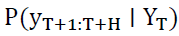 , the distribution of future data points
 , conditional on the currently observed data
 . Reduced form Bayesian Vector Auto regressions usually outperform VARs estimated with frequents techniques (or flat priors). From a more Bayesian perspective, the prior information that may not be apparent in short samples (as for example the long-run properties of economic variables captured by the Minnesota priors helps in forming sharper posterior distributions for the VAR parameters, conditional on an observed sample (Todd, 1984). Mean square error (MSE), root mean square error (RMSE), mean absolute error (MAE) and Theil U statistics were used to assess the forecasting performance. The RMSE and MAE statistics are scale-dependent measures, but allow a comparison between the actual and forecast values. The Theil-U statistics is independent of the scale of the variables and is constructed to lie between zero and one, zero indicating a perfect fit. In evaluating the performance of the forecasting models, the lower the RMSE, MAE, MAPE and Theil-U statistic are better the forecasting accuracy Table 9.
| Table 9 Evaluation of Forecast Accuracy | |||||
| Included observations: 39 | |||||
| Variable | Inc. obs. | RMSE | MAE | MAPE | Theil |
| CPI | 39 | 0.3731 | 0.2822 | 17.875 | 0.1166 |
| IR | 39 | 0.1247 | 0.10441 | 8.4264 | 0.0501 |
| RGDP | 39 | 0.3020 | 0.23589 | 4.45491 | 0.02849 |
| UR | 39 | 0.16272 | 0.12304 | 19.6255 | 0.12755 |
Out of Forecasting Analysis
Based on Table 10, the predicted annual Real GDP growth is increased from 6.2354 in 2018 to 6.2841 in 2019 and the trend in increasing. Similarly the annual Consumer Price Index (inflation) also has increasing trend from 2018 to 2023 but, inflation and Unemployment has a decreasing trend from 2018 to 2023.
| Table 10 Out of Sample Forecast From Bvar (1) | ||||
| Year | LNRGDP | LNCPI | LNIR | LNUR |
| (USD Billion Dollar) | (USD Billion Dollar) | (USD Billion Dollar) | (USD Billion Dollar) | |
| 2019 | 6.28405 | 2.446292 | -1.351825 | 0.70751 |
| 2020 | 6.337459 | 2.497983 | -1.391467 | 0.692156 |
| 2021 | 6.395992 | 2.555675 | -1.42022 | 0.673031 |
| 2022 | 6.459661 | 2.618306 | -1.439215 | 0.652151 |
| 2023 | 6.528232 | 2.684846 | -1.450104 | 0.631047 |
Conclusion
Unemployment, inflation and real GDP growth are co-integrated using Johansson approach and the test suggests that there is long run relationship between unemployment rate and inflation of goods services. Based on the empirical results of pairwise Granger causality test, the study found statistically evidence to conclude that there was direct causality from CPI to RGDP economic growth of Ethiopia. The impulse response function analysis show that shock to RGDP leads to negative response from Unemployment which dies out after four years horizons, while the shock to RGDP from inflation of goods and services produces continuous positive responses. The trend of forecasting using the BVAR, the RGDP and CPI is an increasing trend and the Unemployment has a decreasing trend in the future five years head forecasting. So the government and non-governmental organization should be control unemployment and interest by creating different small enterprise led industrialization strategy and expands the investments for Youth in the country.
Acknowledgement
I am grateful to appreciate one anonymous referee for his guidance, encouraging remarks, patience and positive attitude. Especially his valuable and prompt advice, his tolerance guidance and useful criticism, constructive correction, suggestion and encouragement throughout the progression in preparing the paper are highly appreciated.
Conflict of Interests
The author declares that they have no competing interests.
References
Box, G.E.P., Jenkins, G.M., & Reinsel, G.C. (2008). Time series analysis: Forecasting and control. 4th edn. John Wiely & Sons. Inc, UK ed.
Brewin, J., Nedas, T., Challacombe, B., Elhage, O., Keisu, J., & Dasgupta, P. (2010). Face, content and construct validation of the first virtual reality laparoscopic nephrectomy simulator. BJU International, 106(6), 850-854.
Indexed at, Google Scholar, Cross Ref
Dickey, D.A., & Fuller, W.A. (1981). Likelihood ratio statistics for autoregressive time series with a unit root. Econometrica: Journal of the Econometric Society, 1057-1072.
Indexed at, Google Scholar, Cross Ref
Eden, S. (2012). Modeling inflation volatality and its effects on economic growth in Ethiopia. Addis Ababa University, Ethiopia.
Enders, W. (2008). Applied econometric time series. John Wiley & Sons ed.
Engle, R.F., & Granger, C.W.J. (1987). Co-integration and error correction: representation, estimation, and testing. Econometrica: Journal of the Econometric Society, 251-276.
Indexed at, Google Scholar, Cross Ref
Fama, E.F. (1975). Short-Term interest rates as predictors of inflation. The American Economic Review, 65(3), 269-282.
Indexed at, Google Scholar, Cross Ref
Giannone, D., Lenza, M., Momferatou, D., & Onorante, L. (2014). Short-Term inflation projections: A Bayesian vector autoregressive approach. International Journal of Forecasting, 30(3), 635-644.
Indexed at, Google Scholar, Cross Ref
Johansen, S. (1991). Estimation and hypothesis testing of co-integration vectors in Gaussian. Econometrica, 59(6), 1551-1580.
Johansen, S. (1995). A statistical analysis of cointegration for I (2) variables. Econometric Theory, 11(1), 25-59.
Kaushik, A., Bhatia, Y., Ali, S., & Gupta, D. (2015). Gene network rewiring to study melanoma stage progression and elements essential for driving melanoma. Plos one, 10(11), e0142443.
Indexed at, Google Scholar, Cross Ref
Koop, G., & Korobilis, D. (2013). Bayesian multivariate time series methods for emperical macroeconomics. Foundations and Trends in Economics, 3(4), 267-358.
Litterman, R.B. (1986). Forecasting with Bayesian vector autoregressions-five years of experience. Journal of Business and Economic Statistics, 4(1), 25-38.
Indexed at, Google Scholar, Cross Ref
Mahmood, Y., Bokhari, R., Aslam, M. (2013). Trade-Off between inflation, interest and unemployment rate a cointegration analysis. Pakistan Journal of Commerce and Social Sciences, 7(3), 482-17.
Malam, B., Nwokobia, O.J., Yakubu, K.M., Adama, M.A., & Muhammad, A.A. (2013). Effect of unemployment and inflation on wages in Nigeria. Journal of Emerging Trends in Economics and Management Sciences, 4, 181-188.
Rashid, A., & Kemal, A.R. (1997). Macroeconomic policies and their impact on poverty alleviation in Pakistan. The Pakistan Development Review, 39-68.
Serneels, P. (2004). The nature of unemployment in urban Ethiopia.
Todd, R. (1984). Improving economic forecasting with Bayesian vector autoregression. Quarterly Review-Federal Reserve Bank of Minneapolis, 8.
Todd, R.M. (1990). Vector autoregression evidence on monetarism: Another look at the robustness debate. Quarterly Review-Federal Reserve Bank of Minneapolis, 14(2), 19.
Indexed at, Google Scholar, Cross Ref
Umaru, A., & Zubairu, A.A. (2012). Effect of inflation on the growth and development of the Nigerian economy (An empirical analysis). International Journal of Business and Social Science, 3(10).
Yelwa, M., Okoroafor, O.K.D., & Awe, E. (2015). Analysis of the relationship between Inflation, unemployment and economic growth in Nigeria. Applied Economics and Finance, 2(3), 102-109.
Received: 09-Jan-2022, Manuscript No. JEEER-22-10807; Editor assigned: 12-Jan-2022, PreQC No. JEEER-22-10807(PQ); Reviewed: 25-Jan-2022, QC No. JEEER-22-10807; Revised: 28-Jan-2022, Manuscript No. JEEER-22-10807(R); Published: 02-Feb-2022