Keywords

Crack Price Forecasting, Deep Learning, LSTM, Bayesian Optimizations, Supply Chain Optimization, Oil Refineries.

Introduction

The price difference (gap) between crude oil and refined goods distillates (such gasoline, diesel, jet fuel, etc.) significantly impacts the profit margins of refiners in the petroleum industry (Steven et al., 2014). Since the refining process "Crack" crude oil into its primary refined products, this spread is commonly referred to as the "Crack Spread".

‘Crack Spread’ is of interest to refiners, traders, regulators, hedge funds & speculators, oil market players and academicians (Fousekis & Grigoriadis, 2017). The perspectives and objectives with which they view ‘Crack spread’, however, varies widely. Academic researchers have explored co-integration between petroleum product and crude price, predictive power of crack spread for oil price forecasting, efficacy of day trading strategy for crack spread modelling etc (Poitras & Teoh, 2003). Regulators and International Financial institutions observe crack-spread from the point of view of policy response to market inefficiencies, trade facilitation and regulation of the market. Hedge funds frequently use crack spreads to speculate in oil markets (Murat & Tokat, 2009), and to hedge against refinery stocks or perform directional trade for energy portfolio. Investors can employ crack spread trading as a hedge against the stock value of a refining company. Due to the added benefit of low margins (the crack spread trade generates a big spread credit for margining purposes), other professional traders may think about utilizing crack spreads as a directional trade as part of their energy portfolio. When combined with other indicators such as crude oil stocks and refinery utilization rates, fluctuations in crack spreads or refining margins can offer investors enhanced insights into the future trajectories of specific companies and the broader oil market in the upcoming period. Refiners are exposed to volatility in both the markets in which they operate: crude oil price fluctuations on supply side and volatility in price of refined products in retailing market (Karathanasopoulos et al., 2016). As per (Mahringer & Prokopczuk, 2015), companies engaged in selling crude oil or other products solely to the wholesale and retail markets might face higher susceptibility to market risk compared to refiners. This is as a result of their simultaneous involvement in both markets. (Ederington et al., 2019) contend that numerous factors, such as supply, demand, production economics, environmental restrictions, and other elements, often have individual impacts on the prices of crude oil and its primary refined products.

About 85% (Robinson, 2007) of a typical refining operating cost is made up of crude oil. Because of this, refiners and non-integrated marketers face a significant risk from rising crude oil prices and falling refined product prices on both sides of the market. This can significantly reduce the crack's spread. As a result, executives at refineries are constantly worried about hedging their crack spread risk. With the ability to predict the movement of crack prices well in advance, the refiners can dynamically optimize the right crude-mix through multi-sourcing and development of a compatible hedging strategy for managing the price risk. Refiners seek a return on their invested assets while covering the ongoing and fixed costs of operating the refinery. However, when facing an unpredictable crack spread, refiners find it challenging to assess their actual financial exposure as they can accurately anticipate expenses for everything except crude oil. Oil refiners, therefore, in an effort to optimize the supply chain of oil products, model and predict crack spread with the objectives (Dunis et al., 2016) of (a) Profit maximization by deciding when to procure stocks of crude or processed products (b)Increasing GRM (Gross Refining Margin, or GRM is the difference between the cost of the crude oil used as the input and the total value of the petroleum products that are produced in an oil refinery by selectively choosing crack to process, and (c) Implementing low risk trading / hedging against volatility in crude price fluctuations through futures contracts for protecting the margins. Cracks are thus particularly useful in implementing various procurement strategies and therefore oil refiners have substantial interest in protecting the crack spread (Haigh & Holt, 2002).

Indian Oil Refining and Marketing Companies are more integrated than general oil companies conducting refining and marketing functions in tandem. Therefore, they are not only exposed to the volatility of Crude oil prices arising out of several reasons mentioned earlier but also to inelastic changes in product prices which in turn are impacted by variations in worldwide demand, regional factors, seasonality etc.

Indian Oil refiners import about 85 % of the total required crude oil to meet India’s ever increasing domestic energy demand. The refined petroleum products such as LPG, Petrol, Diesel, Kerosene etc. are sold through the various distribution channels (Dealers, Distributors, Agents etc.) across the country. The profitability of Indian Oil Marketing Companies (OMCs) primarily relies on the cost of imported crude oil and the selling price of products, both of which are linked to international prices as benchmarks. For the purpose of calculating profitability, Indian Oil companies use the prices of Crude from Dubai and prices of products from Singapore exchange.
It has been studied that whereas the Futures of commodities are good forecasts for their spot prices, the same cannot be said for crude and petroleum Crack prices (Reichsfeld & Roache, 2011). Therefore, excellent quality medium term forecasts for Crude and Crack spot prices become the cornerstone of procurement decisions of Indian Oil Companies. State run Indian oil companies have societal obligation to ensure undisrupted supply of fuels across the country. Even in the face of impending unfavourable marketing conditions owing to volatility in crude oil prices, the option to stall operations till favourable return is simply non-existent. Thus, the volatility of crude price and its impact has to be borne out.

With a limited mandate to indulge in financial transactions such as hedging, state run oil companies in India are severely constrained in ensuring profitability and margin protection. In the absence of hedging as an option, Indian state-run oil companies need to resort to forecasted crack spread prices for their procurement planning decisions. The modelling and predicting crack spreads is therefore of greater relevance to refiners for optimizing their supply chain operations and hedging against the volatility in crude oil prices. With reference to the above discussion this study proposes following research questions:

RQ1: How can the crack spread forecast be improved by employing recent advances in Artificial Intelligence and Deep Learning techniques?

RQ2: Can the hybridization of Deep Learning techniques with other popular statistical techniques lead to improvement in forecast accuracy?

RQ3: How can model development and training be optimized by Bayesian optimization?

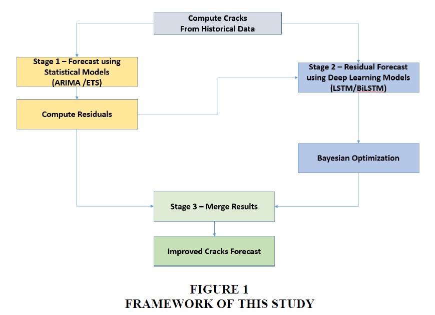
To solve above research questions this study aims to develop a two-stage hybrid model (Figure 1) which will in stage 1 model the linearity present in crack spread time series data using statistical modelling techniques (ARIMA/ETS) and in stage 2 model the non-linearity present in forecast error using non-linear technique such as ANN Deep Learning technique (LSTM/BiLSTM). Also, to optimize the time for development / testing of Deep Learning models, Bayesian optimization is employed. The results of the hybrid model are compared with those of standalone models using metrics namely MSE, RMSE, MAE, MAPE and RMAPE.

Literature Review

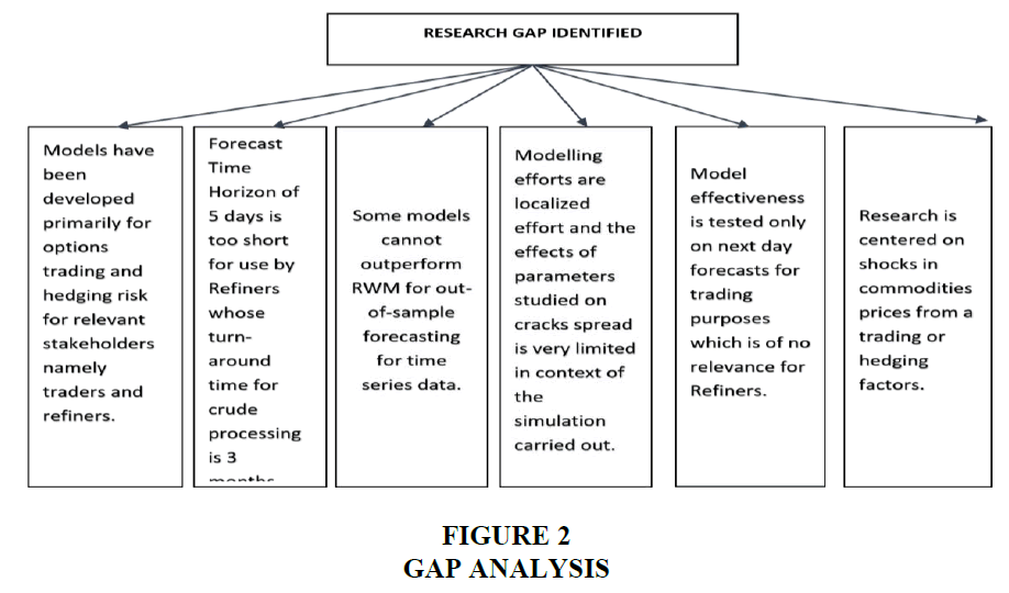
(Karathanasopoulos et al., 2016) utilized a non-linear approach, which integrated a particle swarm optimizer (PSO), a radial basis function neural network, and a sliding window methodology to model and monitor the crack spread. When the model was trained across a 300–400 day sliding window and utilized to produce forecasts for 5 days, it outperformed an MLP neural network in terms of performance and statistical correctness. The forecast time horizon of 5 days though is appropriate for use in trading decision making but is not suitable for Refiners whose turn-around time for procurement-refining-sale of products is 3 months.

High Order Neural Networks (HONN) were used on time series data in a different study on the modelling and trading of gasoline crack spread (Karathanasopoulos et al., 2016) to examine the co-integration between WTI crude and gasoline prices. The method was put to the test in order to forecast how the spread would vary from one closing price to the next. The study did find a non-linear relationship between the price of WTI oil and the cost of gasoline. It is of limited value to refiners because the expected time horizon utilizing the HONN is too short to be regarded a valid fit for the time horizon of three months.

For modelling and forecasting crack spreads have studied ARFIMA (Autoregressive Fractionally Integrated Moving Average) models applied to single product crack. The objective was to verify that crack spread and their volatilities display long range autocorrelation. Also, the study attempted to ascertain that whether crack spreads exhibit multi-fractionality wherein small and large fluctuations exhibit different scaling behaviours. It concluded that Crack spreads exhibited weak mean revering behaviour for time horizon of days and weeks and exhibited strong mean reverting behaviour in weeks and months’ time horizon. On comparison it was found that ARFIMA could not outperform RWM out of sample forecasting and it could not capture the complexity of time series leading to larger prediction bias. ARFIMA could however capture long range autocorrelation but could not capture scaling. Also, it was able to capture multi-fractionality but not small-scale fluctuations.

The multiple regression analysis approach for modelling for naphtha cracking (Sung et al., 2012) looked at the key variables influencing naphtha prices and sought to pinpoint the most important ones. Analyses of naphtha crack's actual and projected variations were also conducted. It was determined that the key factors influencing naphtha pricing were margin, substitutes for naphtha, and supply and demand of naphtha in Asia. For the same, a statistical model was created. In a more recent study by (Ewing & Thompson, 2018), the response of the gasoline-crude oil price crack spread to macroeconomic shocks, such as economic growth, inflation, corporate default risk, and monetary policy shocks, has been analysed and modelled. This method combines a generalized impulse response analysis with a vector auto-regressive approach. Although the results were confined (i.e., pertinent to the specific context of the United States of America), they nonetheless evaluated how shocks to these variables would affect the spread of gasoline crack. The results are listed in Table 1 below.

Table 1 Related Research
Year	Objective	Technique	Findings	Citations
2022	West Texas Intermediate (WTI) oil price patterns are predicted using data from 1991 through 2021.	To ensure model evaluation and comprehensibility, the top-performing machine learning models are assessed and compared using DeLong statistical test methods and SHAP (SHapley Additive exPlanations) values. Among the models in this category are Logistic Regression, Decision Tree, Random Forest, AdaBoost, and XgBoost.	The use of Explainable Machine Learning (XML) models and ML approaches can enhance the forecasting of WTI crude oil prices and have a significant impact on global economic policy.	(H. Guliyev & E. Mustafayev, 2022)
2022	Using news articles, forecast the price of crude oil	With the proposed text indicators, AdaBoost.RT is able to predict crude oil prices better than the other benchmarks with two novel topic and sentiment analysis indicators for short and sparse text data.	An improvement over text indicators based on news headlines and financial characteristics. Sparse and condensed news headlines are used in the framework for forecasting the price of crude oil. These headlines are better suited for price forecasting with historical data.	(Y. Bai et al, 2022)
2022	To develop heuristics for Hedging effectiveness	Comparing two hedging approaches namely minimizing downside risk and minimization of variance in a market exhibiting strong momentum using Copulas based approach	In almost all circumstances (99.6%), the decision-maker's predicted utility is increased by the downside risk minimization hedging strategy. Furthermore, it appears that this method is most effective when both spot and futures prices exhibit strong upward or downward momentum.	(Dmitry Vedenov & Gabriel J. Power, 2022)
2021	Propose a hybrid forecasting model that uses a machine learning algorithm to anticipate crude oil price trends.	The price of crude oil is dissected using a variational mode decomposition technique, and multimodal data features are then retrieved based on the decomposed modes. Time series analysis is used to concurrently translate the volatility of the price of crude oil into trend symbols. Then, multi-modal data features are employed to train a machine learning multi-classifier utilizing historical volatility as input and trend symbols as output.	The hybrid model (ML classification prediction method based on characteristics of multi-modal data) employs the Variational mode decomposition (VMD) algorithm to derive the Intrinsic Mode Functions (IMF) of crude oil prices. Then, multi-modal data characteristics are extracted using the IMFs. It has been proven that the suggested model is more adept at foretelling high volatility than low volatility of crude oil prices.	(He, H., Sun, M., Li, X., et al., 2021)
2021	In the study, the AdaBoost-LSTM and AdaBoost-GRU models are compared to enhance the accuracy of crude oil price prediction.	It introduces the AdaBoost-GRU model, combining the GRU model with AdaBoost Regressor, and compares its predictive power with AdaBoost-LSTM and single LSTM and GRU models.	The results demonstrate that both AdaBoost-LSTM and AdaBoost-GRU outperform benchmarking models, with AdaBoost-GRU showing superior performance compared to all models studied in this research.	(Busari G & Lim D, 2021)
2020	To introduce a robust hybrid model for reliable forecasting of Brent oil price, considering the challenging nature of oil price forecasting.	The proposed hybrid model combines Adaptive Neuro Fuzzy Inference System (ANFIS), Autoregressive Fractionally Integrated Moving Average (ARFIMA), and Markov-switching models to capture specific features in the oil price time series.	The numerical results indicate that the hybrid model weighted by the genetic algorithm performs better than the individual constituent models, the hybrid model with equal weights, and the hybrid model weighted based on error values	(Abdollahi H & Ebrahimi S, 2020)
2018	Determine how the spread of a single product gasoline crack is affected by macroeconomic factors such real production growth, inflation, corporate default risk, and monetary policy stance.	Econometric methods such as Generalized Impulse Response analysis and Vector Auto-Regression (VAR)	Fundamentals in the upstream sector (i.e., unrefined petroleum products) are more responsive to changes in economic production. The crack spread can shift quite significantly in response to small and unexpected changes in aggregate demand. Inflation's effects extend for one to five months. Risk of Corporate Default has no effect. Short-lived monetary policy shocks (up to two months)	(Ewing & Thompson, 2018)
2016	Use a non-linear approach for modelling and tracking the crack's expansion.	The proposed model combines a particle swarm optimizer (PSO) and a radial basis function (RBF) neural network, trained using sliding windows of 300 and 400 days.	The sliding window approach with training periods of 300 and 400 days effectively models the crack spread, while periods of less than 300 days results in performance degradation.	(Karathanasopoulos et al., 2016b)
2016	To forecast the time-series of the WTI-GAS crack spread, use non-linear models.	The best spread trading model is a higher order neural network (HONN) with a threshold filter.	There is a nonlinear relationship between WTI and GAS. Despite faster computation times and fewer variables, HONN fared better than the MLP outside of the sample.	(Dunis et al., 2016)
2015	Comparing pricing of crack spread options using GARCH volatility model or crack spread model.	Time series data for options prices are modelled using bivariate GARCH model and univariate crack spread model	The more simplistic univariate approach to option pricing was found to be better than bivariate GARCH model	(Mahringer & Prokopczuk, 2015)
2014	Systems that facilitate decision-making based on hierarchical planning frameworks are used in the oil refining sector.	Implicit Anticipation model is used to develop a DSS system building on the case study for procurement planning	The case study technique improved the procurement planning for the oil refining industries by resulting in significant reductions in planning efforts and procurement expenses.	(Kallestrup et al, 2014)
2013	To propose a decision support framework that considers the presence of both spot market and contract suppliers to model risks in procurement processes and create a robust purchasing plan.	It introduces the "Expected Profit-Supply at Risk" (A-EPSaR) algorithm, utilizing Monte Carlo simulation to quantify each supplier's risk, allowing decision-makers to understand the trade-off between profit and risk. In addition, a goal programming model to allocate orders among the supplier pool and a contract-spot allocation model to assign orders between the spot market and the supplier pool.	Procurement Risk Management (PRM) framework is designed to support the DSS to identify the risks in the procurement model and build profit model of their own.	(Hong, Z., & Lee, C., 2013)
2013	Predicting the direction of oil price changes	This study proposes a semi-supervised machine learning algorithm (SSL) for time-series entities by representing their network and using SSL to forecast the upward and downward movement of oil prices.	An innovative approach to forecasting oil prices is put forth by adapting the current SSL algorithm for use in time-series prediction. This approach makes use of sophisticated techniques like feature extraction and TI transformation as well as comparisons of the similarity between several collections of time-series data.	(Shin, H. et al, 2013)
2012	For the purpose of modelling and forecasting, verify that crack spread display long range autocorrelation, multi-fractionality and scaling invariance	ARFIMA applied on single product crack	Mean reverting behaviour weak when observed for days & weeks; strong for months, long range multi-fractal with long range autocorrelation but unable to capture small scale fluctuations	(Wang & Wu, 2012)
2012	Create a model for predicting naphtha crack using multiple regression analysis and statistical methods.	Forecasting naphtha crack using a multiple regression model with more than 20 factors	There is a link between naphtha crack and three key affecting elements. Among the main variables, naphtha supply and demand have a significant impact on naphtha crack.	(Sung et al., 2012)
2011	Model the volatility dynamics of the three NYMEX-traded futures contracts for petroleum products (crude oil, gasoline).	The work utilizes the partially overlapping time-series (POTS) framework proposed by Smith (2005) to model all futures contracts with delivery dates up to a year into the future. This approach allows the extraction of information from these prices to understand the persistence of market shocks.	The findings reveal time-to-delivery effects, substantial seasonality, and variations in conditional variance and correlation across the commodities, with implications for short-term and one-year price risk in different positions, particularly in crack-spread positions.	(Suenaga & Smith, 2011)
2010	The paper explores the use of data mining techniques for stock market prediction.	It proposes combining three well-known feature selection methods, namely Principal Component Analysis (PCA), Genetic Algorithms (GA), and decision trees (CART), to identify more representative variables for better prediction.	The results show that the best-performing combinations of feature selection methods are the intersection of PCA and GA, and the multi-intersection of PCA, GA, and CART, achieving accuracies of 79% and 78.98%, respectively.	(C.-F. Tsai & Y.-C. Hsiao, 2010)

Forecasts utilizing crack spread option pricing were examined using 2 different approaches in a study by (Mahringer & Prokopczuk, 2015). Option 1 employed a two-factor mean-reverting model with constant volatility to simulate the crack spread option. On the other hand, Option 2 utilized a bivariate GARCH model with co-integrated underlying futures to model the crack spreads between crude oil and heating oil, and crude oil and gasoline.

In analysing the price risk to crack spread due to volatility dynamics and seasonality (Suenaga & Smith, n.d.) modelled using econometric techniques the shocks to prices of crude oil Gasoline and heating oil. This study attempted to factor in the impact inventory held (Geman & Smith, 2013)and the maturity of futures contract. The three commodity prices' highly nonlinear volatility dynamics were shown by the estimated model, which is in keeping with the seasonality in storage and demand that has been observed. Despite the fact that all three commodities have sizable seasonal changes and time-to-delivery impacts, there are notable variances between the three commodities' volatility patterns and the contract's delivery month.

The price discovery process for petroleum products, how accurately petroleum product futures prices predict current spot prices, and refinery outages and weather were all identified as important fundamental factors in a survey on the factors influencing the prices of petroleum products (Ederington et al., 2019). The empirical findings led to the conclusion that, throughout the study period, speculation did not lead to an increase in risk-free returns on petroleum products or in excess returns or price volatility. Studies reveal that gasoline and heating oil futures prices are often reliable indicators for three-month spot prices, but not as much for six and 12-month contract durations. When assessed for forecasting performance, gasoline futures prices outperform a simple random walk (by producing less mean-squared errors) and perform better than both oil and heating oil futures in this regard.

To develop heuristics for Crack spread hedgers, the study by (Liu et al., 2017) compared two hedging strategies namely minimizing the downside risk criterion and minimization of variance measure on Expected Utility. The study found that the downside risk minimization hedging strategy increases the expected utility of the decision-maker to almost 99.6% of the time. Moreover, this approach works best when both spot and futures prices move upward and downward strongly Tables 1 & 2.

Table 2 Performance Measures
Variance		Accuracy
Variance

This research attempts to address the identified gaps (Figure 2) by developing a model for forecasting price of single product crack spread with horizon of 1-3 months using crude and product benchmarks used by Indian refiners using time series data and employing recent advances in AI Deep Learning techniques.

Time Series Modelling: Statistical Machine Learning Models

Auto Regressive Integrated Moving Average (ARIMA) models are a powerful tool for forecasting time series data. They are used to forecast a wide variety of data, including sales, economic indicators, and environmental data. A comparison of various statistical and machine learning techniques has been developed for generating forecasts (Makridakis et al., 2018). ARIMA models, or Autoregressive Integrated Moving Average models, are a class of statistical models that are used to analyze and forecast time series data. ARIMA models assume that the future values of a time series can be predicted from its past values and the errors of its past predictions.

ARIMA models have been used for reliability forecasting and analysis (Ho et al., 2002). The time series technique is a forecasting technique that requires no assumptions about the data and is very flexible (Burba, 2019). An improvement of ARIMA model is the SARIMA model which includes more realistic dynamics of data specifically non-stationary in mean and seasonal behaviours (Gerolimetto, 2010). Since time series forecasting analysis can be conducted only on stationary data, differencing (by taking logarithm) is carried out to convert data from non-stationary to stationary(Ho et al., 2002). The non-stationary data is subjected to order of differencing (d=0,1,2) to make it stationary (Bhardwaj et al., 2014). The traditional ARIMA model does not incorporate impact of external independent variables. Exogenous variables can be incorporated in the ARIMA (Jain & Mallick, 2017) and SARIMA (Gerolimetto, 2010) models which will incorporate effects of any external variables which exhibit regressive relationships to the base model (Xie et al., 2013).

Time series data are also typically forecasted using the ETS method, also known as the Holt-Winters method . The model effectively captures the errors, trends, and seasonality of a time series and can be applied to both univariate and multivariate data. Generally, the error component of an ETS is the random fluctuations that occur in a time series of data. ETS can improve forecast accuracy by incorporating historical errors into its forecasting model.

In time series data, the trend component represents the long-term pattern or direction. Trends can be captured by estimating the slope and incorporating it into the forecasting model, which will project future values that align with the overall direction of the data. Data series that repeat at regular intervals, such as daily, weekly, or yearly, are said to be seasonal. ETS can provide accurate predictions for future values by estimating seasonal indices and applying them to the forecasting model.

Deep Learning Models

An LSTM is a type of Recurrent Neural Network that is used in Deep Learning applications. Because it can identify patterns in both short-term and long-term input sequences, LSTM in particular is well suited to categorizing, evaluating, and making predictions. A typical example will be sequence of words in a sentence or patterns in time series data wherein we are unsure of the patterns / lags that may exist in the sequence / data series (Gu et al., 2019; Salvi, 2019; Siami-Namini & Namin, 2018; Song et al., 2020).

LSTMs can keep contextual information on input sequences by providing a loop through which information can flow from one stage to another. An LSTM unit consists of a cell, an input gate, an output gate, and a forget gate. LSTM were developed to address RNN's vanishing gradient problem, which is brought on by backpropagation. They still experience the exploding gradient problem, though. An extension of the traditional LSTM is the Bi-directional LSTMs (BiLSTM) which improves the performance of sequence classification problems (Siami-Namini et al., 2019). Two hidden layers pointing in different directions are connected to the same output by LSTMs. In this type of degenerative learning, the output layer is simultaneosly given knowledge about both the past and the future states. This aids the LSTM in comprehending the situation more fully (Kulshrestha et al., 2020). The LSTMs come in a variety of flavours, including vanilla, stacked, bi-directional, CNN, and conventional. The study makes use of and contrasts these tastes.

Bayesian Optimization

The process of determining the ideal collection of hyperparameters in deep learning and machine learning which control the learning process is called as hyper parameter optimization. Some of the most commonly used algorithms are Grid Search, Random Search, and Bayesian Optimization. Bayesian optimization uses an automatic model tuning approach to fine tune the hyperparameters. This method uses a surrogate model, such as Gaussian Process for approximating the objective function. During this optimization, two choices are made:

1. Choosing previous functions to optimize that express assumptions about the function. In this case, we pick the Gaussian Process.

2. The acquisition function must be chosen.

Evaluation Metrics for Models

As is customary in the literature, the provided forecasts are statistically analysed using the Mean Squared Error (MSE), Root Mean Squared Error (RMSE), Mean absolute error (MAE), Mean absolute percentage error (MAPE) (Karathanasopoulos et al., 2016).

For comparison of models, we have also employed and additional measure for accuracy Resistant-MAPE (R-MAPE) in our study which is a better fit (Table 3) for comparing accuracy of time series models(Montaño Moreno et al., 2013).

Table 3 Comparison of MAPE and R-MAPE
Characteristic	MAPE	R-MAPE
Sensitivity to outliers	More sensitive	Less sensitive
Interpretability	Easier to interpret	More difficult to interpret
Suitability for different applications	Good for forecasting applications where the actual values are relatively similar in magnitude	Good for forecasting applications where the actual values vary widely in magnitude or where there are outliers
Examples of applications	Forecasting sales for individual products in a retail store	Forecasting demand for electricity or water

Acceptable levels of MAPE and RMSE for a time series forecasting model vary depending on the specific application and the industry. However, in general, the following guidelines can be used:

MAPE: A MAPE of 10% or less is generally considered to be highly accurate, while a MAPE of 20% or less is considered to be good. MAPE between 20% and 50% is considered reasonable. A MAPE of greater than 50% is generally considered to be poor or inaccurate forecasting (Montaño Moreno et al., 2013) .

RMSE: The acceptable level of RMSE for a particular application may be higher or lower depending on the specific needs of the business (Shcherbakov et al., 2013). Additional factors that should be kept in mind to consider when evaluating the reasonableness of RMSE for demand forecasting:

• Frequency of the forecasts: More frequent forecasts (e.g., daily or weekly) will generally have higher RMSE than less frequent forecasts (e.g., monthly or quarterly). This is because more frequent forecasts are more difficult to predict accurately.

• Level of aggregation: Forecasts for more aggregated data (e.g., total demand for a product category) will generally have lower RMSE than forecasts for less aggregated data (e.g., demand for a specific product). This is because aggregated data is less noisy and easier to predict.

• Horizon of the forecasts: Forecasts for shorter horizons (e.g., next week or next month) will generally have lower RMSE than forecasts for longer horizons (e.g., next year or next five years). This is because shorter-term forecasts are less subject to unexpected changes in the environment. An RMSE that is less than or equal to the standard deviation of the historical data is generally considered to be good. An RMSE that is greater than the standard deviation of the historical data is generally considered to be poor. This bodes from the fact that the standard deviation of the historical data is a measure of how much the data varies. If the RMSE of a forecast is less than or equal to the standard deviation of the historical data, then it means that the forecast is at least as good as the historical average. However, if the RMSE of a forecast is greater than the standard deviation of the historical data, then it means that the forecast is not as good as the historical average. For comparative studies, the model with the least RMSE measure will be the best option.

Data Description

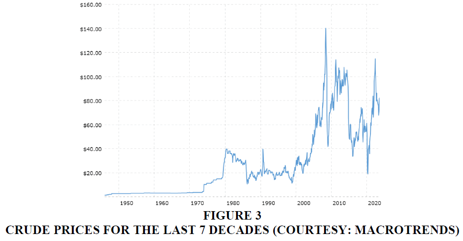
The price of Crude oil has undergone tectonic shifts during the past few decades. The following Figure 3 depicts the price of Crude Oil from 1980s till date.

The volatility (rise and fall) and major shifts in price levels are clearly discernible and attributable to major events such as Gulf War (1990-91), The Y2K Bubble (1998-200), Sub-prime lending crisis in USA (2008), Excess shale gas production by US (2014-15) and the COVID-19 pandemic in 2020 to name some of the few major events. If for the purpose of model development and training the complete set of data ranging from 1990 till date is used, then it will result in models which wrongly would factor extraneous events and their implications which have no systemic bearing in forecasting of the prices of Crude and products for operational purposes. To exclude the extreme effects of such drastic shifts in prices owing to extraneous events as outlined above, data for this research has been chosen from the window corresponding to June. 2015 till Dec 2019. During this period, there is an absence of any political, economic or any such event and the prices are purely reflective of the market dynamics namely the demand, supply, and prices.

Data Selection

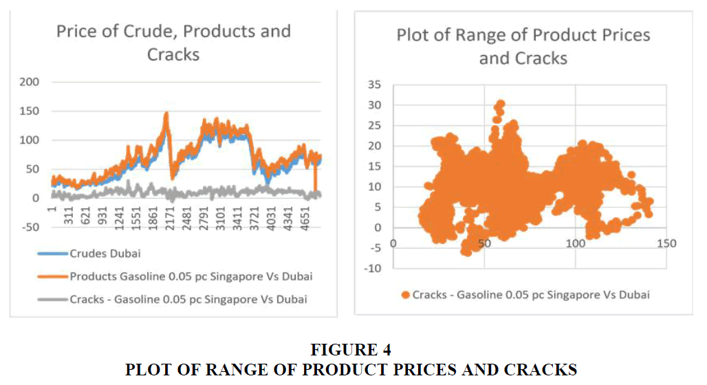
This research uses data sourced from daily feeds provided by Platts comprising of all types of traded Crude and Petroleum products. For the purpose of model development, Brent Crude oil prices and Gasoline 0.05 % Singapore prices have been used. The prices for the Crude and Products are plotted in USD $/Barrel in Figure 4. The price of crack spreads on a given day is determined by subtracting the difference between the daily closing product prices in US dollars from the price of crude in US dollars. Whereas for the purpose of planning and GRM calculation, various crack spreads namely the 5:3:2 and 3:2:1 crack spread are used. The 5:3:2 Crack spread denotes that 5 units of Crude oil is used to produce 3 units of Gasoline and 2 units of Gas oil. The GRM is thus calculated basis on the yield (i.e., percentage of Gasoil and Gasoline produce per gallon of Crude oil and computed proportionately. However, for the purpose of simplicity of model development only one Product (Gasoline) has been used to calculate the gasoline crack based on Brent Crude oil prices. This scenario closely reflects the reference crude and product prices being used by Indian Oil companies. The model so developed can be easily extended to other crack spread combinations if so desired.

Data from the training set make up 80% of the total, whereas data from the test set make up 20% of the total.

Data Pre-processing

A time series could have missing and irregular numbers. Using appropriate method, the noisy data are smoothed, and the missing values are replaced. Heteroscedastic data is when a time series' dependent variable significantly varies from the beginning to the end of the series. By taking the time series' logarithm, heteroscedastic behaviour can be eliminated.

In order to assess the predictability of time series crack spread data is used, the ADF statistics for the crack time series data is computed and is listed below Table 4.

Table 4 ADF Statistics for Crack Spead Time Series Data
S.No.	Parameter	Value
1.	ADF Statistics	-6.160728
2.	p-Value	0.0000
3.	Critical value of 1%	-3.432
4.	Critical Value of 5 %	-2.982
5.	Critical Value of 10%	-2.567

During the deep learning training process, data is standardized. When the actual forecasts are generated at the end of the modelling process, this process is reversed. The Google TensorFlow framework and various Python libraries like Keras, Pandas, etc. are utilized to implement the deep learning techniques employed in this study. The kerastuner software serves as a foundation for the Bayesian optimization-based hyperparameter training for Deep Leaning and Optimization Model.

Modelling

The available dataset is divided into two halves for the purpose of training the LSTM models, with the training set comprising 80% of the data and the testing set the remaining 20% the testing set When building and training the LSTM network, various hyperparameters are used in addition to the lag size parameter, including the number of hidden layers, epoch size, batch size, number of neurons, learning rate, and dropout rate. In the following stage, an LSTM network is built and trained using the training set that corresponds to each set of hyperparameters that was valued using Bayesian optimization in the previous stage. The grid search method is used to turn the time series into a set of instances with an input-output format based on the lag size that is chosen. An example of the produced instances with lag size = 10 is shown in Table 5. After that, a train set and a test set are created from the instances that were produced. The test set comprises 20% of all the examples in each experiment. An LSTM network is constructed and trained for each combination of hyperparameters. The Adam algorithm serves as the optimizer for all networks (Kingma & Ba, 2014). Furthermore, the mean squared error (MSE) is utilized as the loss function for every constructed LSTM network. The final crack price forecast is arrived at by adding the forecast obtained in stage (1) with the residual forecast obtained in stage (2). The performance of the model so developed is computed based on the prevalent error metrics and using the metrices Mean, Variance, Standard Deviation, Mean Square Error (MSE), Root Mean Square Error (RMSE), Mean Absolute Error (MAE), Mean Absolute Percentage Error (MAPE) and Resistant-MAPE (R-MAPE).

Table 5 Comparison of Errors Between Statistical ARIMA, ETS Deep Learning (MLP/LSTM/BILSTM) Models
	ARIMA	ETS	MLP	LSTM	BiLSTM
VAR	6.78	6.72	17.01	11.06	5.87
SD	2.60	2.59	4.12	3.30	2.42
MSE	6.84	6.77	30.61	14.72	6.15
RMSE	2.63	2.66	5.52	3.88	2.60
MAE	2.24	2.23	3.87	3.00	2.03
MAPE	35.29	35.21	49.27	112.97	47.04
RMAPE	29.21	29.31	48.39	119.64	43.71

Result and Analysis

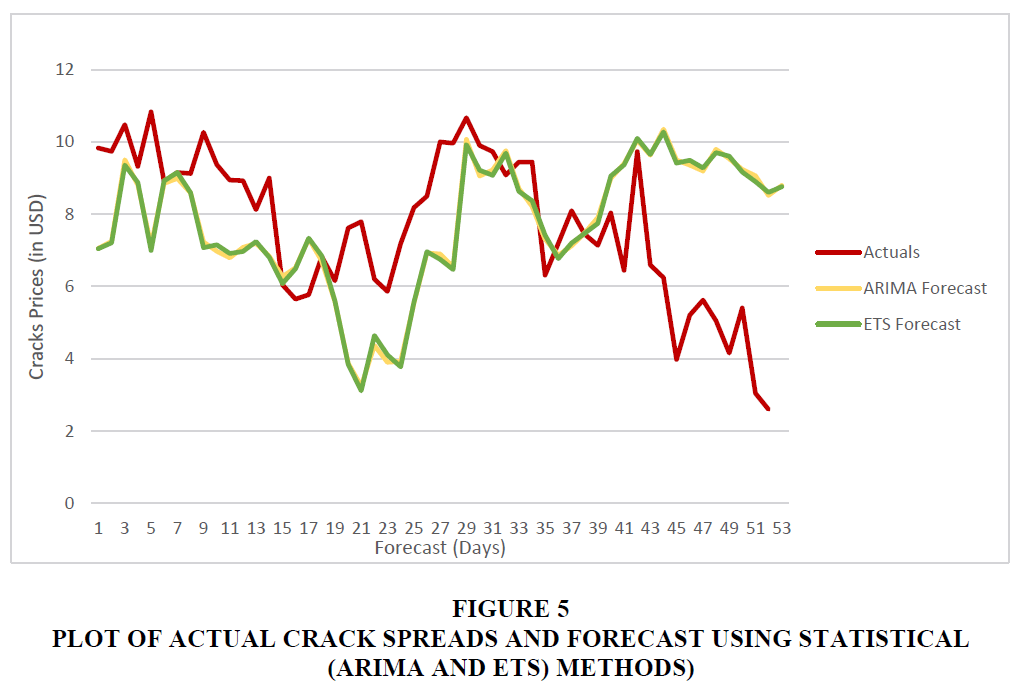
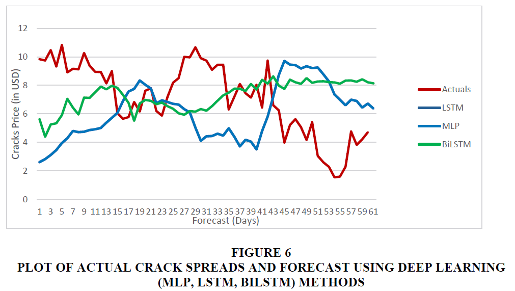
As a baseline, forecasts were computed using statistical models namely ARIMA, ETS and ANN Deep Learning models namely MLP, RNN models LSTM and BiLSTM.

As is evident from Figure 5 above, the forecasts computed using statistical techniques ARIMA and ETS denote similar behaviour.

However, forecasts generated using deep learning methods MLP, LSTM and BiLSTM (Figure 6) are exhibit different behaviour.

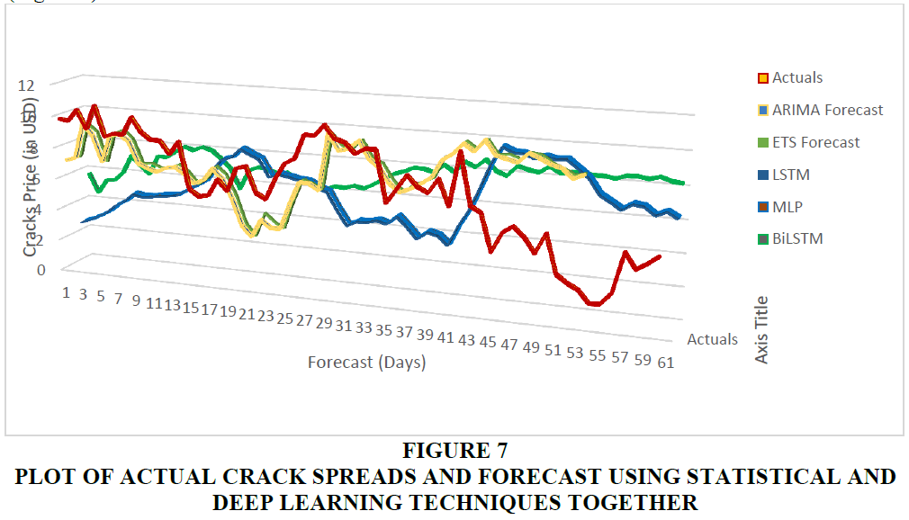
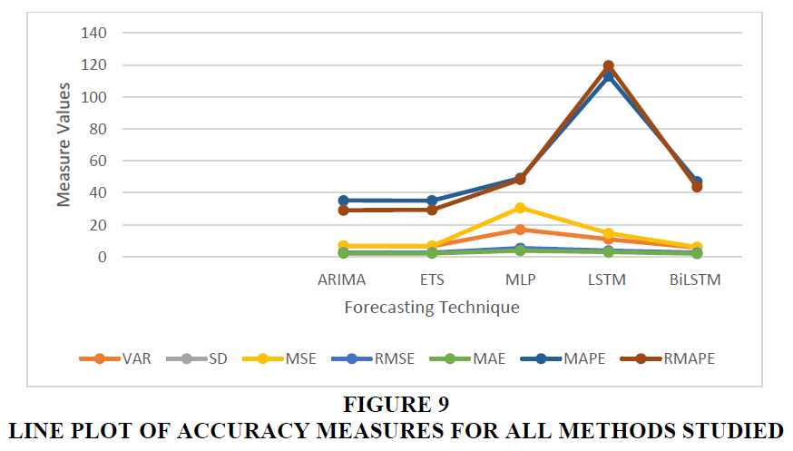
A combined plot of Actual crack spread and forecasts using all the techniques under study is plotted in Figure 7 above. The tabulation of performance metrices related to these forecasts is provided in Table 5 below.

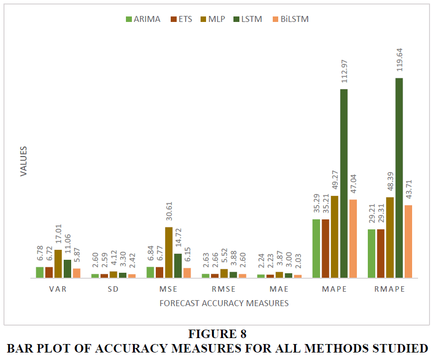
It can be inferred from the table above that ARIMA and ETS methods provide a very similar performance amongst the statistical techniques but the performance of deep learning methods varies considerably. BiLSTM exhibits the best performance amongst the deep learning techniques and exhibits better MSE and RMSE. However, its MAPE / RMAPE performance is inferior to ARIMA and ETS methods. On an individual basis ETS, LSTM and BiLSTM have RMSE scores less than their Standard Deviation, meaning that they are generating better forecasts. Viewed from the perspective of MAPE / RMAPE none of the methods when considered individually produce good quality forecasts (i.e., their individual MAPE / RMAPE are greater than 20).

Bar plots and Line plots of the various metrices are provided in Figures 8 and 9 above.

To improve the forecasting method, as mentioned in the earlier section of this paper, we have taken ARIMA and ETS both as statistical method and BiLSTM method as the deep learning technique for further studies.

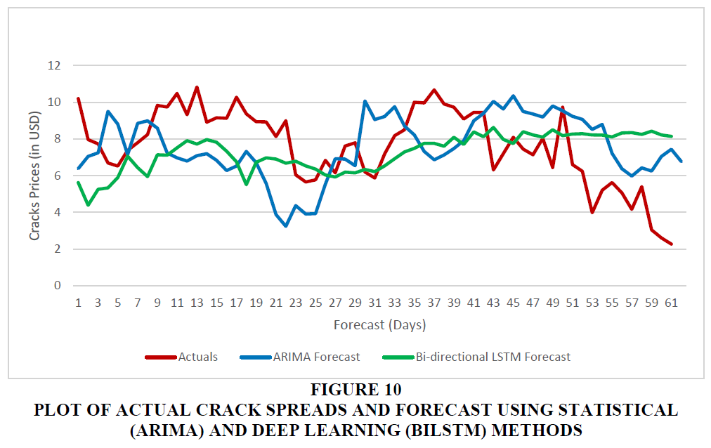
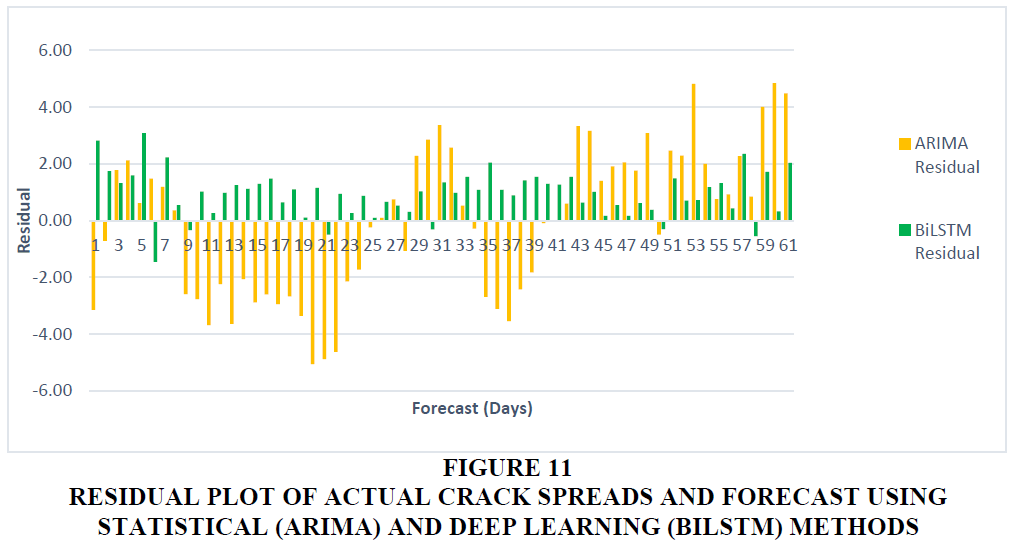
Figures 10 and 11 provide comparison of ARIMA and BiLSTM forecasts plotted side by side. The results of 2 stage forecasts using ARIMA and ETS for stage 1 and BiLSTM for forecasting residuals in Stage 2 and finally calculating the forecasts are listed in Table 6 below.

Table 6 Comparison of Errors between ETS+LSTM and Hybrid LSTM Models
	ARIMA	BiLSTM	ARIMA + BiLSTM Residual	ETS	ETS + BiLSTM Residual
VAR	6.78	5.87	2.26	6.72	2.78
SD	2.60	2.42	1.50	2.59	1.67
MSE	6.84	6.15	2.25	6.77	2.80
RMSE	2.63	2.60	1.50	2.66	1.66
MAE	2.24	3.00	1.26	2.23	1.39
MAPE	35.29	112.97	19.89	35.21	23.54
RMAPE	29.21	119.64	16.4	29.31	18.61

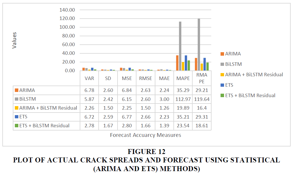
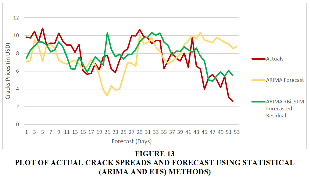
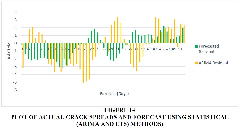
We observer there is a considerable improvement in forecasts using ARIMA + BiLSTM when compared to using ARIMA, ETS and BiLSTM individually. The RMSE score of the ARIMA + BiLSTM is less than the SD and MAPE RMAPE scores are also less than 20, which is the threshold for the quality of the forecasts to be considered good.

Figure 12 plots all the observed scores for this combination of forecasting.

Figures 13 and 14 provide a comparison plot of ARIMA and ARIMA + BiLSTM forecasts.

Ranking of the Various Models (Standalone and Hybrid)

The Table 6 provides the ranking of all the models standalone (ARIMA, ETS, MLP, LSTM, BiLSTM) and hybrid models ARIMA+ BiLSTM and ETS + BiLSTM models. The performance metrices in the order of significance are MAE, RMSE, RMAPE and MAPE Table 7.

Table 7 Ranking of Crack Spread Forecasting Models
Model	Standard Deviation	MAE Score	RMSE Score	MAPE Score	RMAPE Score	Rank
ARIMA+BiLSTM	1.5	1.26	1.5	19.89	16.4	1
ETS+BiLSTM	1.67	1.39	1.66	23.54	18.61	2
BiLSTM	2.41	2.03	2.6	47.04	43.71	3
ETS	2.59	2.23	2.66	35.21	29.31	4
ARIMA	2.6	2.24	2.63	35.29	29.21	5
LSTM	3.3	3	3.88	112.97	119.64	6
MLP	17.01	3.87	5.52	49.27	48.39	7

A combination of statistical forecasting technique ARIMA and BiLSTM for forecasting the price of crack offers the best performance. This approach brings together the forecasting strengths of two techniques namely ARIMA, a statistical technique which addresses well the linearity present the data and BiLSTM, a deep learning method, which captures the non-linearity present in the data. Combining these techniques yields improvement in the accuracy of the forecast beyond what each of the techniques individually yield.

Hyper Parameter Tuning

Hyperparameter tuning using Bayesian optimization offers significant improvement in training times in comparison to other methods of optimization like Random search and Grid search. The best results are obtained with 4 Dense Layers, Epoch =10 and activation function = ‘relu.

Discussion

Crack spread forecasting is less researched a topic as compared to Crude price forecasting. Most of the existing research on Crack spread forecasting is oriented towards short term forecast with a horizon of few days and is primarily intended for Traders and hedge fund managers. Various techniques such as Vector Auto Regression, Multiple regression, neural networks, General Brownian Motion and ARFIMA have been employed for the purpose of forecasting crack spreads. Time series analysis has been the dominant technique adopted for most of the research on crude oil and crack spread forecasting. On visual examination, it can be deduced that the Crack spread timeseries has both linear and non-linear component. Any technique employed which is primarily aimed for modelling either the linear or non-linear component for forecasting will invariably be unable to capture the nuances of the other component. This is evident in the results discussed earlier in this paper.

This research attempts to develop a hybrid model for improving forecast accuracy which employs statistical forecasting technique ARIMA for forecasting the linear component and ANN Deep Learning BiLSTM model for forecasting the non-linear component. This study is based on and extends a similar approach proposed by (Panigrahi & Behera, 2017) by employing Deep Learning LSTM in place of the Multi-Layer Perceptron (MLP) to the domain of crack spread forecasting. For comparison, various Deep Learning Architectures have been studied for hybridization and the results were obtained with BiLSTM. The results indicate that this hybridization results in generation of forecasts with better accuracy compared to individual methods which model linear or non-linear components, respectively.

Theoretical Implications

Deep Learning techniques have a history of success when employed in pattern recognition applications like image categorization, self-driving automobiles, and similar ones. The Multi-Layer Perceptron (MLP), Convolution Neural Network (CNN), and Recurrent Neural Networks (RNN) Deep Learning architectures all perform differently for a given set of tasks, though Long Short-Term Memory (LSTM) neural networks, a type of RNN, are known to perform better on short and long sequences of input streams in contrast to other Deep Learning Neural Network Architectures. This study also performs a comparative study of performance of all these Deep Learning architectures on Time Series data, Crack spreads prices in this case and we observe a behaviour congruent on the stated lines i.e., BiLSTM models perform better than MLP and classical LSTM models. Bayesian optimization has been used to increase the rate of convergence of models and has been found to be effective when in reducing run times for large combinations of model and their configurations. This study can also be extended to include crude / crack futures which are also represented as time series and combination of these series can be expected to increase the efficacy of forecast still better.

Managerial Implications

The crude oil constitutes 85% of the input cost of refinery operations. Indian Oil companies, unlike their western counterparts, are integrated oil refining and marketing companies. With limited options to engage in pricing of petroleum products and limited mandate to engage in hedging as a safeguard, managers in Indian oil companies are left with limited options to improve their profitability. Oil refineries procure and process a ‘basket of crude’ depending upon the design of the refinery to process a particular type of crude (sweet / sour crude), the configuration of the refinery for producing various distillates (LPG, Gasoil, etc.) and suitable alternatives of crude available at a lesser cost among other factors. The crude(s) thus selected amongst the alternatives available by comparing the forecasted Crack spreads for each of the available options and ensuring the highest forecasted crack spreads can immediately lead to increase in cost optimization and profitability as measured using Gross Refining Margin (GRM). The calculation for computing the impact of unit percentage improvement in forecast accuracy to GRM is convoluted, however rough estimates indicate that it can lead to increase in around 0.1- 0.2 % annual profit for Indian Oil refining and marketing companies amounting to approximately 20-40 crores annually. Crack spread forecasts with higher accuracy, therefore, becomes central to this theme. This improvised and easy to implement method therefore provides a robust and inexpensive way for generating crack spread forecast with higher accuracy to Managers of Oil companies to aid their planning and procurement decisions.

Conclusion

Practicing managers involved in the supply chain planning and optimization of petroleum products have always felt the need for superior quality forecast of petroleum product prices (crude, distillates / crack) as it has direct bearing on GRM hence profitability. In order to improve forecasting accuracy, we have attempted to create a hybrid model that combines statistical modelling technique ARIMA with Deep Learning technique BiLSTM. The linearity present in the time series data allows the ARIMA technique to be used to estimate the price of a sole product crack. By utilizing the LSTM Deep Learning technique to extract more information from the nonlinearity of the residuals, the forecast accuracy is boosted. A variety of LSTM single and hybridized mode combinations have been researched and ranked according to their efficacy. Bayesian optimization was used to expedite the hyper parameter tuning procedure. The ANN models are thus able to converge faster to optimal hyper-parameters for the Deep Learning networks employed. This study therefore establishes that hybrid models which combine statistical and AI techniques yield better results. This work can be extended to study the effectiveness of these steps for multi-step / period forecasting. Also, various newly discovered ANN Architectures such as Autoencoders, Transformers and DeepAR etc. which can be studied to ascertain the improvement in the forecast accuracy. Combining these techniques with other optimization techniques such as Portfolio optimization techniques can lead to sustained profitability for the organizations. The recent advances in development of Artificial Neural Network ecosystems such as GPUs and TPUs, Programming Languages and Machine Learning libraries, also accelerate the research in various areas of petroleum products demand and their price forecasting, and supply chain planning. This study has implemented a hybrid model, which combine statistical techniques such as ARIMA and ANN Deep Learning techniques, namely BiLSTM networks, to capture both linearity and non-linearity in time-series data and make more accurate short-term forecasts. This study is however limited to univariate time series and short terms forecasts. As a future extension to this study, the following enhancements can be attempted i) The hybrid model comprising of ARIMA, and LSTM can be extended for medium- and long-term forecasts ii) Study and analyse the performance and effectiveness of these model for multistep forecasting iii) Other deep learning models such as Boltzman machine (Deep Belief Network) / transformers have yielded better results when coupled with LSTM deep learning models iv) use a portfolio approach to create the ideal combination of Deep Learning models for various forecasting horizons; v) Application of Generative AI (such as ChatGPT etc. ) for time series forecasting vi) investigate the effects of bagging on ARIMA models and hybrid models. vi) Research into hyperparameter tuning methods using Bayesian optimization.

References

Bhardwaj, S. P., Paul, R. K., Singh, D. R., & Singh, K. N. (2014). An Empirical Investigation of Arima and Garch Models in Agricultural Price Forecasting. Economic Affairs, 59(3), 415.

Indexed at, Google Scholar, Cross Ref

Burba, D. (2019). An overview of time series forecasting models. Towards Data Science, 1–20.

Dunis, C. L., Laws, J., & Evans, B. (2016). Modelling and trading the gasoline crack spread: A non-linear story. Derivatives and Hedge Funds, 12(1), 140–160.

Indexed at, Google Scholar, Cross Ref

Ederington, L. H., Fernando, C. S., Hoelscher, S. A., Lee, T. K., & Linn, S. C. (2019). A review of the evidence on the relation between crude oil prices and petroleum product prices. Journal of Commodity Markets, 13(9), 1–15.

Indexed at, Google Scholar, Cross Ref

Ewing, B. T., & Thompson, M. A. (2018). Modeling the Response of Gasoline-Crude Oil Price Crack Spread Macroeconomic Shocks. Atlantic Economic Journal, 46(2), 203–213.

Indexed at, Google Scholar, Cross Ref

Fousekis, P., & Grigoriadis, V. (2017). Price co-movement and the crack spread in the US futures markets. Journal of Commodity Markets, 7(8), 57–71.

Indexed at, Google Scholar, Cross Ref

Geman, H., & Smith, W. O. (2013). Theory of storage, inventory and volatility in the LME base metals. Resources Policy, 38(1), 18–28.

Indexed at, Google Scholar, Cross Ref

Gerolimetto, M. (2010). ARIMA and SARIMA models and ARIMA. 1, 1–5.

Gu, Q., Lu, N., & Liu, L. (2019). A novel recurrent neural network algorithm with long short-term memory model for futures trading. Journal of Intelligent and Fuzzy Systems, 37(4), 4477–4484.

Indexed at, Google Scholar, Cross Ref

Haigh, M. S., & Holt, M. T. (2002). Crack spread hedging: Accounting for time-varying volatility spillovers in the energy futures markets. Journal of Applied Econometrics, 17(3), 269–289.

Indexed at, Google Scholar, Cross Ref

Jain, G., & Mallick, B. (2017). A Study of Time Series Models ARIMA and ETS. SSRN Electronic Journal.

Indexed at, Google Scholar, Cross Ref

Karathanasopoulos, A., Dunis, C., & Khalil, S. (2016). Modelling, forecasting and trading with a new sliding window approach: the crack spread example. Quantitative Finance, 16(12), 1875–1886.

Indexed at, Google Scholar, Cross Ref

Kulshrestha, A., Krishnaswamy, V., & Sharma, M. (2020). Bayesian BILSTM approach for tourism demand forecasting. Annals of Tourism Research, 83(4), 102925.

Indexed at, Google Scholar, Cross Ref

Liu, P., Vedenov, D., & Power, G. J. (2017). Is hedging the crack spread no longer all it’s cracked up to be? Energy Economics, 63(4), 31–40.

Indexed at, Google Scholar, Cross Ref

Mahringer, S., & Prokopczuk, M. (2015). An empirical model comparison for valuing crack spread options. Energy Economics, 51, 177–187.

Indexed at, Google Scholar, Cross Ref

Makridakis, S., Spiliotis, E., & Assimakopoulos, V. (2018). Statistical and Machine Learning forecasting methods: Concerns and ways forward. PLoS ONE, 13(3), 1–26.

Indexed at, Google Scholar, Cross Ref

Montaño Moreno, J. J., Palmer Pol, A., Sesé Abad, A., & Cajal Blasco, B. (2013). El índice R-MAPE como medida resistente del ajuste en la previsionn. Psicothema, 25(4), 500–506.

Indexed at, Google Scholar, Cross Ref

Murat, A., & Tokat, E. (2009). Forecasting oil price movements with crack spread futures. Energy Economics, 31(1), 85–90.

Indexed at, Google Scholar, Cross Ref

Panigrahi, S., & Behera, H. S. (2017). A hybrid ETS–ANN model for time series forecasting. Engineering Applications of Artificial Intelligence, 66(7), 49–59.

Indexed at, Google Scholar, Cross Ref

Poitras, G., & Teoh, A. (2003). Trading & Regulation Volume Nine Number Two 2003 Derivatives Use. In Trading & Regulation (Vol. 9, Issue 2). Henry Stewart Publications.

Reichsfeld, D., & Roache, S. (2011). Do Commodity Futures Help Forecast Spot Prices? IMF Working Papers, 11(254), 1.

Indexed at, Google Scholar, Cross Ref

Robinson, P. R. (2006). Petroleum processing overview. In Practical advances in petroleum processing (pp. 1-78). New York, NY: Springer New York..

Google Scholar

Salvi, H. (2019). Long Short-Term Model for Brent Oil Price Forecasting. International Journal for Research in Applied Science and Engineering Technology, 7(11), 315–319.

Google Scholar, Cross Ref

Shcherbakov, M. V., Brebels, A., Shcherbakova, N. L., Tyukov, A. P., Janovsky, T. A., & Kamaev, V. A. evich. (2013). A survey of forecast error measures. World Applied Sciences Journal, 24(24), 171–176.

Google Scholar, Cross Ref

Siami-Namini, S., & Namin, A. S. (2018). Forecasting economics and financial time series: ARIMA vs. LSTM. arXiv preprint arXiv:1803.06386.

Google Scholar

Siami-Namini, S., Tavakoli, N., & Namin, A. S. (2019). A comparative analysis of forecasting financial time series using arima, lstm, and bilstm. arXiv preprint arXiv:1911.09512.

Google Scholar, Cross Ref

Song, X., Liu, Y., Xue, L., Wang, J., Zhang, J., Wang, J., Jiang, L., & Cheng, Z. (2020). Time-series well performance prediction based on Long Short-Term Memory (LSTM) neural network model. Journal of Petroleum Science and Engineering, 186, 106682.

Indexed at, Google Scholar, Cross Ref

Steven, L., Taylor, G., Daniel, A., & Tolleth, M. (2014). Understanding Crude oil and Product Markets. American Petroleum Institute, 4, 1–39.

Suenaga, H., & Smith, A. (n.d.). Volatility Dynamics and Seasonality in Energy Prices: Implications for Crack-Spread Price Risk. The Energy Journal, 32(3).

Indexed at, Google Scholar, Cross Ref

Sung, C., Kwon, H., Lee, J., Yoon, H., & Moon, I. (2012). Forecasting Naphtha Price Crack Using Multiple Regression Analysis. Computer Aided Chemical Engineering, 31(7), 145–149.

Indexed at, Google Scholar, Cross Ref

Xie, M., Sandels, C., Zhu, K., & Nordstrom, L. (2013). A seasonal ARIMA model with exogenous variables for elspot electricity prices in Sweden. International Conference on the European Energy Market, EEM.

Google Scholar, Cross Ref

Received: 09-Oct-2023, Manuscript No. AMSJ-23-14021; Editor assigned: 10-Oct-2023, PreQC No. AMSJ-23-14021(PQ); Reviewed: 29-Dec- 2023, QC No. AMSJ-23-14021; Revised: 29-Feb-2024, Manuscript No. AMSJ-23-14021(R); Published: 02-Mar-2024