Keywords

Yield, Education, Investment, Wage, Regression, Inequality.

JEL Classifications

E24, I21, J24, J31.

Introduction

The formulation of the earnings function of Mincer (1961) is the starting point of a large literature that has studied the evaluation of returns to education. the other studies have tried to take better understand how the present and past environment of an individual affected the returns to education and the differences in the educational choice between individuals synthesized in particular by Card (2001), and especially by using the instrumental variables which allows to take into account the endogeneity of certain explanatory variables Ahmad & Butt (2012); Hungerford & Solon (1987).

However, the literature that we consulted did not reveal any typology of the consequences of depreciation or the associated models explaining the mutual relationship between the possible effects (Weeks et al., 2004; Neuman & Weiss, 1995; Van Loo & Semeijn, 2005; Shearer & Steger, 1975; Thijssen, 2005; Laureys, 2014; Nazarov et al., 2018).

The objective of this paper is to present the empirical analysis of the earnings mode l from three investigations, which will be limited, first, to only educational investments. This model is the approximation of the general model. Secondly, we develop a descriptive statistic, and thirdly, the simple schooling model will be extended through the introduction of professional investment Becker & Chiswick (1996). Two types of regression will be presented, that describe the behavior of individuals towards post-school investment. The first is linear, and the second is exponential, in order to measure in a robust way the return of the various educational investments and to test whether there is a depreciation effect or not.

During each step, we will try to compare the different results of different Surveys while respecting the same comparison framework Altonj & Pierret (2001).

Statistical data is provided by three surveys carried out by the NSI (National Statistics Institute) the Survey 1 done in 1989, which includes after cleaning 7549 people, the Survey 2 done in 1999 contain 5896 people, and the Survey 3 carried out in 2012 which includes 63078 people. And for the estimations we use the Gretl software (Fitzgerald et al., 1998).

Methods/Experimental

This work can be designed to bring value or less in five areas:

Methodologically, where he respects strict scientific standards as a professional in the field, this work oscillates between the traditional guideline and the new trends, where we have tried throughout this article to be faithful to a strict scientific structuring while carrying our specific style and leaving a distinctive character on the manuscript.

On the knowledge level, the study can be considered as a reference in what relates to the theory of education yield, even that the latter is relatively recent and a little delicate, the present study brings new conceptions while respecting the spirit general of the formulation resulting from the theory.

On the innovative level, the analysis postulates, to our knowledge, new innovative avenues, even if we note that the approach is aimed at specialists in the field, the sequence of ideas allows readers to understand the objective as well as the results.

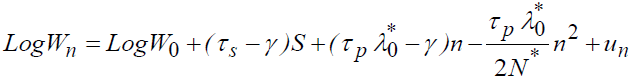
This article reviews the Mincer model, thus specifying a new formulation, centered on the depreciation of the human capital.

The reformulation respects the framework of the human capital theory and tries to answer the questions of contemporary society, particularly concerning the return on school and professional investments.

On a practical level, the study is interesting from the point of view that it demonstrates the simplicity and delicacy of the treatment of the effect of return on investment while respecting the characteristics of the economy to be studied, where we took the example of Tunisia.

The study makes it possible to understand the evolution of the returns schools' and professional investments, to look for points of failure and disequilibria in the education system, and the relationship with the labor market. In addition, the study can be assessing the impact of government policy concerning educational policies and programs.

Processing of Survey 1

Methodology: The Simple Schooling Model

This model is an approximation of the general model of Mincer, which makes it possible to write the natural logarithm of the wages "Log(Y0)" according to the number of years of study "S", we will test these two functions. The addition of the variable "S²" in the second regression allows us to deduce the marginal contribution of education for different levels of education.

The results of the regressions are as follows¹:

The coefficient "α1" is not significant in the regression "2", the average rate of return to schooling is 5.19%, and we note that the coefficient "α2"associated with the square of the education variable is positive, which imply that the return to education increases as the level of education increases. Besides, according to regression "2", we can write:

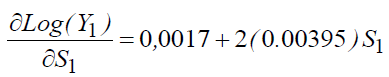
So for S₁=6 (primary education) we will have τ (the yield)=4.91%

For S₁=9 ⇒ τ=7.28%, for S₁=13 ⇒ τ=10.44%

For S₁=17 ⇒ τ=13.6%

Note that the multiple correlation coefficients are relatively low, so the education variable only explains 19.7% of the first regression and 22.5% if we introduce the second explanatory variable. This is due to the basic specification of the simple schooling model.

We can improve the prediction by adopting the catch-up design (Overtaking). The study consists of testing an education model, the salary of which corresponds only to the educational investment, which corresponds to the gross salary at entry into working life. However, the problem is that grosses wages are not directly observable.

Since that the gross salary is higher than the net salary (especially at the start of working life), and the increase of the grosses salary is less than that of the net wage. At some point, the net wage catches up with the initial level of the gross salary, so if we recover this threshold, the estimate of the wage that corresponds to it will be much better.

Most studies estimate that the catch-up period will be between 7 and 9 years of working life. We will test the simple education model, taking special account of this restriction; the number of observations will be reduced to 892 people.

The results are as follows:

Comparison of these results with those of the previous regression, where we estimated the model using all the observations, we notice that the average rate of return on school investments doubled from 5.19% to 10.33%. The coefficient of "" is not significant, which confirms the first approach stating that the return to education increases as the level of education rises.

We also note that the multiple correlation coefficients have improved significantly from 22.5% to 43.22%, showing that a more precise quantification of educational investment allows more robust estimates.

Empirical Analysis Including Professional Investments

To analyze the evolution of salaries according to the level of training and by age group, we have grouped the employees according to four levels of training:

1. None: education equal to zero,

2. Primary: from 1 to 6 years of study,

3. Secondary: from 7 to 13 years of study,

4. Higher: more than 13 years of study.

We distinguish 13 age groups, the extent of each group being four years. The same classification will be adopted when treating the salary according to the number of years of professional life.

We, therefore, analyze the age-logarithm profiles of wages, and the number of professional years-logarithm profiles of wages (we always calculate the average of the logarithms of wages for each group).

We can write the variation of the logarithm of the net salary for the period "n" and "n + 1" in the form²:

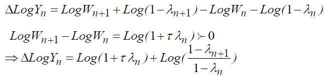
This explains that the variation of the logarithm of the net salary depends on "Log (1 + τ λn)" and that the concavity is ensured by the decrease of "λn" with age.

The concavity shows that the decrease in "λn" is faster for those with low educational levels than for high levels.

Characterization of the Equations to be estimated

In this section, we will test the earning model that only generates educational and professional investments, where we define two cases:

The case without depreciation:

The case with depreciation:

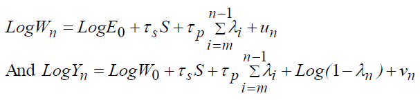
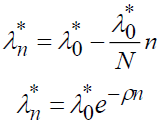
With Wn: the gross salary, Yn: the net salary, S: the number of years of schooling, τs: the average rate of return on educational investments, τp: the average rate of return on professional investments, γ : the average rate of depreciation of human capital, λn : the fraction of the salary allocated to professional investment, : the fraction of gross salary allocated to gross investment, "m": the time of entry into working life, n: the number of years of professional life, and N: the total length of the period of net investment.

We are going to adopt two regressions that retrace individual behaviors for post-school investment³.

The first regression is linear: 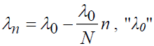explains the part of the gross salary intended for investment during the first period of working life.

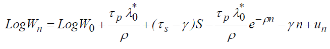
The second regression: 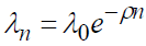this expression develops the exponential decrease in the part of the salary intended for investment, of parameter "ρ".

Characterization without Depreciation

Using the linear form in the previous model, we will have:

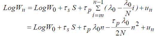
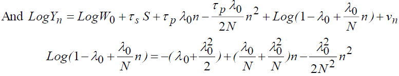
Taylor's quadratic approximation gives:

Therefore:

(1)

There is a parabolic relationship between the logarithm of wages and the time spent in working life.

Using the exponential form, the model will be as follows:

The expression of the net salary is:

The same Taylor's quadratic approximation gives:

(2)

(Function of Gompertz's salary).

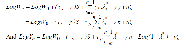
Characterization with Depreciation

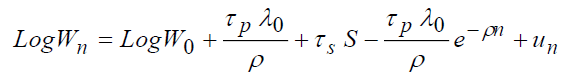
By introducing the depreciation effect, we will have:

Introducing the first investment specification into the gross wage equation gives:

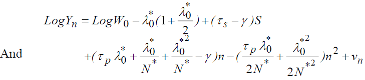(3)

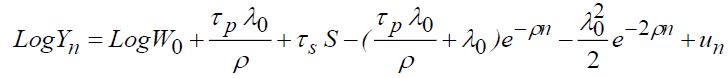
The second gives:

We can, therefore, deduct the net salary:

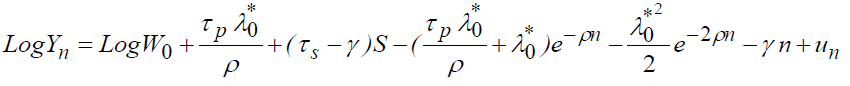(4)

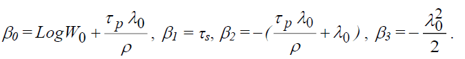
For the econometric study, we only use the equations which describe the net salary: (1), (2), (3), (4). We estimate the specifications proceeding in the linear form (1) and (3) by the following equation:

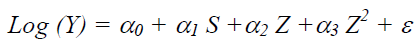
Knowing that, S: number of years of study, Z: number of years of professional life, Z²: square of Z.

For the specification without depreciation, the coefficients of the equation are defined such that:

And with depreciation:

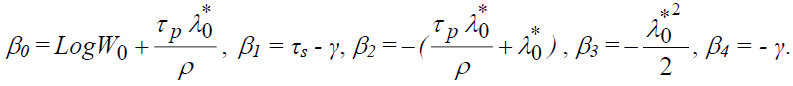
Then, we estimate the specifications proceeding in the exponential form ((2) and (4)) by the following equation:

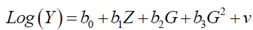
Knowing that, G=e^-ρn and G2=e^-2ρn

Without depreciation, the coefficients of the equation are defined such that:

With depreciation:

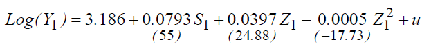
Result of the Estimates

R²=29.63%.

1. We note that all the variables are significant for all the models.

2. The introduction of the variable "Z1" in the model improves the explanatory power of the regression, where we note that the multiple correlation coefficients go from 19.7% to 26.7%.

3. Taking into account the variable "Z1" partly eliminates the bias that affected the estimation of the rate of return to education. This bias is explained, on the one hand, by the short professional life of the most qualified at the same age, on the other hand, by the increase in the average level of education of the population. This explains a biased estimate of the rate of return on educational investment.

4. The introduction of the variable " " corrects the average rate of return on school investment, which is around 7.93% (instead of ‎‎5.19%).

The calculation of marginal rates of return on school investments makes it possible to write:

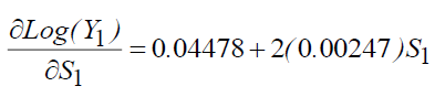
This means that for:

S1=6 (Primary education) we will have τs (The yield) =7.44%

S1=9 ⇒ τs=8.92%, S1=13 ⇒ τs=10.9%,

S1=17 ⇒ τs=12.87%.

There is an increase in returns for all levels of education, except for the higher level, there is a decrease. It should be noted here that the classic pattern of diminishing marginal returns is not respected because these returns increase with the level of education.

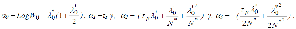
The calculation of the profitability of professional investment goes through the calculation of "α2" and "α3". Besides, we know that:

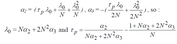
We also know that "λ0" is between zero and "1", which places restrictions on the choice of "N" (the total length of the investment period)

According to regression (2) we obtain the following results:

For N=20 ⇒ λ0 =39.54% and τp =3.08%,

N=25 ⇒ λ0 =36.92% and τp =5.29%,

N=30 ⇒ λ0 =29.31% and τp =9.25%.

We can therefore estimate that the returns to professional investments in the Tunisian economy are low.

The cumulative duration of professional investments is:

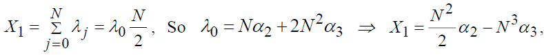the condition of maximization of X1 give 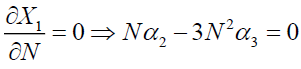, for N?0 we will have

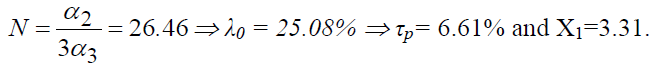
The cumulative duration of on-the-job investments is at its maximum for N =26.46; its time equivalent is, therefore, equal to 3.31. When "N1" is maximum, the fraction of the salary intended for professional investors will be 0.25; the rate of return corresponding to this placement is 6.61%.

Finally, we note that the sign of the interaction variable "SZ1" which is the product of the variable "S1" and the variable "Z1", is negative which reflects a convergence of salary profiles and years of professional life.

The Results of the Gompertz Function Estimate

The advantage of this method is to provide all the necessary information without having to resort to other transformations or extrinsic variables:

R²=29.45%.

The value taken for "ρ" is 0.0615 (other regressions were made for different values of "ρ", but we only keep the good one, the one that increases the "R²" and that the coefficients are significant).

The estimate shows that the average return on education has not changed (around 7.9%).

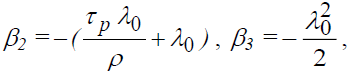so from "β3" we can calculate "λ0", and of "β2" we deduce "τp", so we will have λ0=69.01% and τp=0.44%.

The study of depreciation refers to the regression of model 4, where the variable "Z1" is introduced (the coefficient of this variable expresses the rate of depreciation of human capital during working life).

Hence γ =0.91%. We note that this coefficient is negative and significant. So, we will have: τs=β1+γ=0.0799+0.0091=8.9%.

Processing of Survey 2

The Simple Schooling Model

The estimation of the model gives the following results⁴:

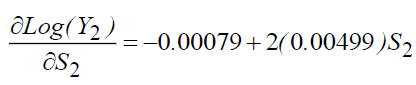
The return to education stands at 6.48%, an improvement of almost a point in a decade (5.19% in 1989). We note that in the second regression the coefficient of "S₂" is not significant for a threshold of 5%, however, the multiple correlation coefficients is improved, going from 31.6% to 34.7%.

The calculation of marginal returns gives:

Therefore, we can write:

S2=6 (primary education) we will have τs (the yield) = 5.9%

S2=9⇒ τs = 8.9%, S2=13⇒ τs=12.89%,

S2=17⇒ τs=16.88%.

The comparison of the different returns with those of the first survey shows that, on the one hand, the marginal returns always increase with the increase of the years of study; on the other hand, there is an improvement in these yields for all levels. However, the greatest increase is recorded for the upper level (from 13.6% to 16.88%).

The estimation of the model by referring to the principle of Overtaking and always adopting as a catch-up period between 7 and 9 years of professional life allows more solid estimates. Consideration of this specification, the sample will be reduced to 558 people.

The results will be as follows:

These estimates show an improvement in the return to education (from 6.48% to 9.35%), but this increase is less than that recorded at the time of the study of the first survey (from 5.19% to 10.33%), which indicates a bad signal concerning the contribution of education to returns. On the other hand, we note a clear improvement in the level of explanatory power which climbs to 52.09%.

Empirical Analysis with Professional Investment

In this section, we will use the same study principle as that adopted for the Survey1 (four levels of education, thirteen age groups, range of four years, and we calculate the average of the logarithms of wages for each group).

We have found that at the same age we always have the logarithm of the salary of the most educated is higher than that of the less educated. This observation is approved during working life, especially between primary and secondary level, and between secondary and higher level. We can distinguish two stages, the first is characterized by a narrowing of the crack between the two levels up to the period 38-41 years, and the second phase marks a divergence. We also notice that these profiles are neither flat nor parallel (describing the presence of an investment other than education).

Note that the concavity is clearer for the lower levels than for the upper levels, and the decrease in "λn" is always higher for the lower levels than for the higher levels, which explains the widening of the slot between the gain profiles of the different levels.

Finally, we note that the maximum of the earning profiles is reached at the end of the career for the upper and secondary levels, and a little less for the other two levels.

The study highlights the following observations:

1. We have two stages of professional investment (with an equal duration of professional life). The first stage is marked by a tendency to catch up with the least educated levels, explained by a greater professional investment; the second stage is marked by the predominances of higher Professional investments from the most educated.

2. It can also be seen that the trend line of the upper levels is almost linear; however, this phenomenon was recorded for lower levels during the survey study 1. The other curves have a concave shape.

3. The most educated individuals have a shorter professional life.

4. At the start of a career, salaries are different between the different levels

Estimation of the Equations

Parabolic Function

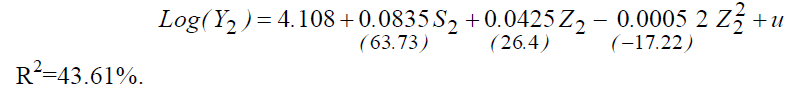
All variables are significant for all models, except the variables "Z₂" and "SZ₂" in Model 2.

It should also be noted that introducing the variable "Z₂" improves the explanatory power of the model (40.78% instead of 31.6%), since the introduction of this variable partially eliminates the bias that affected the rate of average return on education.

Switching to the full model by inserting the square of "Z₂" readjusts the average rate of return on educational investment from 6.48% to 8.35%. Compared with the Survey 1, we can detect a slight improvement over a decade (by 0.42%).

The study of marginal returns to schooling brings out (Model 4):

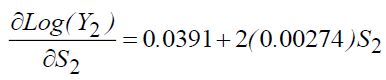
So, we can write:

S2=6 (primary education) we will have, τs (the yield) = 7.2%

S2=9 ⇒ τs =8.84%, S2=13 ⇒ τs=11.03%,

S2=17 ⇒ τs =13.23%.

These results show that there is an increase in marginal returns compared to the simple model, except for the top level. But we can notice by comparing the returns of the two surveys, that the marginal returns of the lower levels recorded a decrease during these 10 years, and an increase in yields for the upper levels (from 12.87% to 13.23%), implying a tendency to value the high levels at the expense of those of the low level. But this trend remains weak.

Regarding professional profitability and regarding model "2" gives:

For N=20 ⇒ λ0=43.07% and τp=2.72%,

N=25 ⇒ λ0=40.72% and τp=4.81%,

N=30 ⇒ λ0=33.12% and τp=8.4%.

We can conclude that at "N" equal, the "λ0" has increased since the Survey 1, which means that the agents increased their post-school investments, but on the other hand, the profitability decreased. Thus, for a decade, people have invested more and earned less.

According to Model 2, the interaction variable "SZ₂" is not significant, which does not allow us to distinguish the relationship between education and experience.

The cumulative duration of post-school investments is:

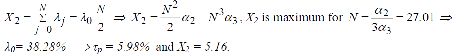
The cumulative duration of professional investments reaches its maximum for X=27.01; its time equivalent is, therefore, equal to 5.16. If "X2" is maximum, the fraction of the salary spent on on-the-job investment will be 0.382. The rate of return equivalent to these expenses is 5.98%.

Comparison of these figures with those of 1989 shows that there is an increase in "N", "λ0" and "X" but a decrease in " τp".

The Gompertz Function Estimate

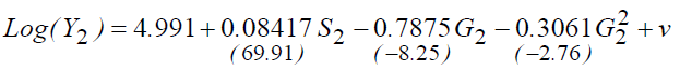
R²=43.86%.

It can be noted that there is no change in the profitability of education, if we compare this model with that of the basic model, using parabolic regression. Likewise, the observed difference is always the same if we compare the estimation results of the two surveys.

The chosen value of "ρ" this time is 0.066, so λ0=78.24% and τp=0.0427%. Likewise, here we can deduce an increase in professional investment, while their profitability of this investment decreases if we compare the results of the two surveys, under the Gompertz regression.

Regarding the state of depreciation, we can refer to the coefficient of the variable "Z₂" in the model 4, where we record γ = 1%, the coefficient is negative and significant; therefore, the phenomenon of the depreciation of human capital during working life is justified. Moreover, we note that this rate has increased compared to the Survey 1.

The gross profitability of education is, therefore:

Processing of Survey 3

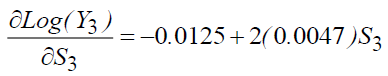
The Simple Schooling Model

The estimate shows the following results⁵:

We noted that the average return on education has deteriorated to 5.98% (against 6.48% in 1999). The calculation of marginal returns makes it possible to give:

And therefore:

S3=6 (primary education) we will have τs (the yield)=2.63%

S3=9 ⇒ τs=5.2%, S3=13 ⇒ τs=8.63%,

S3=17 ⇒ τs=12.05%.

We can find that marginal returns always increase with the number of years of schooling. However, the comparison of these results with those of the Survey 2 shows a decrease in these returns for all levels, primary, secondary, and higher (degradation of two points for each level)⁶.

Estimating the model by limiting itself to a professional life between 7 and 9 years (Overtaking) reduces the sample to 5,454 people, which gives the following results:

These estimation results show an improvement in the average return to education ranging from 5.98% to 9.8%, almost the same rate recorded for the Survey 2. But it is still lower than the return to education for Survey 1 (under the same conditions). However, there is a marked improvement in the explanatory power of the model.

Empirical Analysis Including Professional Investments

In this section, we will use the same grouping procedure as when processing the two previous surveys, in order to allow reliable and consistent comparisons between the different surveys.

The first finding that can be raised is the one related to the pace of earnings profiles, where we can see a clear improvement compared to the two previous surveys.

At the start of working life, the profiles are almost the same except for that of the higher level. Then, they will be well distinguished towards the end of working life. However, these profiles were clearly distinguished from the start for the other two surveys.

At the same age, the most educated people have higher earnings profiles than the less educated. And this pattern will be sustained over the course of working life with an increasing and continuous rhythm, of which the possibilities of catching up for low levels are almost nil (attempts recorded during the study of surveys 1 and 2).

The concavities of the profiles in this survey are checked for all levels of training. The concavity will be compared to the decrease in "λn" as the age increases; this decrease is more severe for low levels.

The logarithm of wages peaks when workers cross the 54-57 age range. It can be seen that the most educated have a shorter professional life than the others. We also note that the most educated allocate larger sums to professional investment, which still confirms the positive correlation between school and post-school investments. But the comparison with the other two surveys shows that the most educated are spending less and less of their spending on professional investment. This is explained by the declining return distinguished over time from professional investment.

Estimation of the Equations

Parabolic Form

The estimation of the model gives:

R²=39.67%.

The study of the outputs of the estimates shows that all the variables are significant, we also note that the insertion of the variable "Z3" and "Z₃²" increases the explanatory power of the model (39.67%) and the average yield of the educational investment which goes from 5.98% to 8.34%.

The comparison of these rates with those of the Survey2 indicates a slight decrease in the average return to education, which confirms the decrease already observed since the Survey1 for the valuation of educational investments.

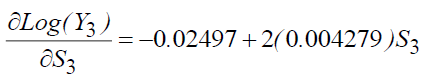
Marginal returns to education are calculated from the Model 2:

The marginal returns from the different levels of education are thus:

S3=6 (primary education) gives τs (the yield) =4.39%

S3=9 ⇒ τs =7.22%,

S3=13 ⇒ τs =10.99%,

S3=17 ⇒ τs =14.75%.

We note an increase in marginal returns compared to the simple schooling model, with a rate of almost two points for each level of education. Comparison of these results with those of Survey 2 reveals a decrease in marginal returns for all levels of education, with the exception of the case S3=17, and the conclusions already identified during the study of Survey 2 can be confirmed the gold of the Survey 3 study.

In terms of the profitability of professional investments, we can calculate for different values of "N", from model 2:

For N=20 ⇒ λ0=43.1% and τp=2.38%,

N=25 ⇒ λ0=41.66% and τp=4.19%,

N=30 ⇒ λ0=35.33% and τp=7.11%.

If we compare the results of the three surveys, we notice that for "N" equal, "λ0" has been increasing since the 1989 survey, which shows that people are attaching more and more importance to the post-school investment. However, profitability continues to decline.

The interaction variable "SZ₃" has a positive and significant coefficient, which indicates that there is a complementary relationship between formal education and post-school training.

The cumulative duration of professional investments is:

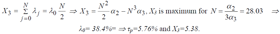
The maximum of the cumulative duration of professional investments is reached for "N =28.03" for a time equivalent "X3=5.38", the part of the salary allocated to the investment professional is therefore 0.384, with a rate of return equal to 5.76%.

We note that reaching the optimum, and comparing it with the values found during the processing of Survey 1 and 2, is characterized by an increase in the investment period "N", the share of income spent on investment "λ0" and of "X", on the other hand, there is a decrease in profitability "τp". This builds contradictions in the economy.

Gompertz Function Estimate

R²=39.88%.

We can notice that the returns to schooling, as well as the explanatory power of the model have not changed compared to the basic model with a parabolic regression. However, the estimate shows that the return to average education decreased compared to the Survey 2 according to the Gompertz specification.

In this case, the value of "ρ" chosen is equal to 0.058. We can, therefore, notice that the "ρ" chosen for the three surveys is around 6%.

So, λ0=40 8% and τp=7.62%. Consequently, we can say that this generation has benefited from the benefits of the professional investments of previous generations (error in the memory of generations) since the proportion "λ0" devoted to post-school investment decreases while profitability increases compared to the Survey 1 and 2 in part of this model.

The inclusion of the variable "Z3" in model 5 makes it possible to deduce the value of the depreciation coefficient γ =1.27%, which is negatively significant. So, there, once again, the phenomenon of the depreciation of human capital is justified. Moreover, it has been increasing since the Survey 1.

We can, therefore, deduct the average return on education without depreciation (gross return):

If we compare the gross return on the education of the three surveys, we can see a slight increase ranging from 8.9% in 1989 to 9.41% in 1999 to stabilize at 9.64% in 2012.

Results and Discussion

In terms of results, throughout the study, we tried to draw results beyond the classical formulations by specifying the necessary demonstrations.

The analysis makes it possible to compare the output of the estimate based on three job surveys using a new conception of the Mincer model, thus dissecting the factors that influence the decision-making process.

The returns on education and professional investments thus deduced allow comparisons to be made and their development to be sketched out.

Limits, the main limitation lies in the possibility of adopting instrumental variables (still to prove the validity) for the estimation, which can be the subject of future research under the basis of this new specification with depreciation.

Conclusion

Our construction of a gain function inspired by HC models made it possible to satisfactorily understand the returns on investment in training by overcoming the shortcomings observed in the Mincer formulation and by adopting three NSI surveys.

However, it was found, during the processing of the 1989 survey, that the average internal return to education in the simple schooling model is 5.16%, while it is 10.33% if we correct using the catch-up method, reaching 7.93% in the full model with post-school investment. Estimating the Gompertz function also gives similar results, yielding 7.99%.

Concerning the 1999 survey, the simple education model gives a return of 6.48% and with the conditions of catch-up amounts to 9.35%, while it is 8.35% in the model including professional investments. Likewise, the Gompertz function estimate confirms the complete model with a rate of return of 8.41%.

Examination of the 2012 survey shows a rate of return of 5.98% in the simple model. The catch-up specification makes it possible to identify a rate of return which amounts to 9.8%, whereas it is 8.31% in the case of the addition of professional investment, a rate which is confirmed by Gomert'z sttimate which shows a rate of 8.36%.

By comparing these different rates in the different cases, it can be seen that overall, the average internal return to education is deteriorating.

Besides, the study of the dynamics of marginal returns to education also shows a depreciation of returns for all levels of education.

The coefficient of the depreciation variable expresses the rate of depreciation of human capital during working life. However, the study shows that this coefficient is negative and significant.

We can see that marginal returns always increase with the number of years of schooling. However, the comparison of these results from the different surveys shows a decrease in these returns for all levels, primary, secondary and higher since 1989 (deterioration of two points for each level).

We also adopted two regressions that track individual behaviors for post-school investment. A linear regression explains the share of the gross salary intended for investment during the first period of working life and an exponential expression which describes the decrease in the share of the salary intended for investment during the second phase.

This specification partially eliminates the bias that affects the estimation of the rate of return to education. This bias is explained, on the one hand, by the fact that at the same age the most qualified have shorter working lives, on the other hand, by the increase in the average level of education of the population.

The study shows low returns on professional investments in the Tunisian economy. We note also that the sign of the interaction variable is negative, which implies a convergence of the profiles of wages and years of professional life.

We also note that the most educated allocate larger sums to professional investors, which traces a positive correlation between school and post-school investments. But these allocated sums have become weaker and weaker for more than two decades.

Analysis of the results of the three surveys shows that for the same total duration of the investment period, the fraction of the salary intended for professional investors has increased since the 1989 survey, which shows that people are paying more and more importance to post-school investment, However, profitability continues to decline.

We can therefore see that the period 1989-2012 is marked by an increase in the period of professional investment as well as the share of income devoted to this investment, however, there is a decrease in post-school profitability which creates contradictions in the labor market.

The immediate recommendation is to fight against the devaluation of diplomas, by rethinking the reform processes from planning to decision-making, reconsidering the university map in-depth, and creating an integrated development tool that respects the training levels.

Conflicts of Interest

The author declares that this article does not include any conflicts of interest, either potential or apparent.

Declarations

1. Ethics approval and consent to participate: Not applicable

2. Consent for publication: Not applicable

3. Availability of data and material: The data supporting the results of this study are available from [National Institute of Statistics (NIS)] but restrictions apply to the availability of these data, which have been used under license for this study, and are therefore not accessible to the public. Data are, however, available from the authors upon reasonable request and with permission from [NIS].

4. Competing interests: Not applicable

5. Funding: Not applicable

6. Authors' contributions: All authors have read and approved the final manuscript

7. Acknowledgements: Not applicable

8. Authors' information: Not applicable

List of Abbreviations

Log (Y0) = α0: The basic minimum wage.

S: The number of years of schooling.

S2: Square of S.

α1: The average rate of return of educational investments.

Log (Y): the logarithm of wages.

τ : The yield.

λn: The fraction of gross wages allocated to investment.

Wn: Gross earnings.

Yn: The net earnings.

En: Expenses.

Wn: The gross salary.

Yn: The net salary.

τs: The average rate of return on educational investments.

τp: The average rate of return on professional investments.

γ : the average rate of depreciation of human capital.

λn : The fraction of the salary allocated to professional investment.

λ*n : The fraction of gross salary allocated to gross investment.

m: the time of entry into working life.

n: The number of years of professional life.

N: The total length of the period of net investment.

ρ: The part of the salary intended for investment.

G = e^-ρn: Specifications proceeding in the exponential form.

Z: Number of years of professional life.

Z²: Square of Z.

X1::The cumulative duration of professional investments

End Notes

1. Student statistics appear in parentheses under the coefficients.
The index "1" means Survey 1.
The outputs of the estimation software are available from the author.

2. λn= En / Wn the fraction of gross wages allocated to investment.
Wn: Gross earnings.
Yn: The net earnings.
En: Expenses.

3. The demonstrations that come are specific to the author.

4. Student statistics appear in parentheses under the coefficients.
The index "2" means Survey 2.

5. Student statistics appear in parentheses under the coefficients.
The index "3" means Survey 3.

6. The comparison with Survey 1 shows a decrease in marginal returns by one point for each level of education.

References

Ahmad, S., & Butt, M.M. (2012). Can after sale service generate brand equity. Marketing Intelligence & Planning.

Indexed at, Google Scholar, Cross Ref

Altonj, I., & Pierret, C. (2001). Employer learning statistical discrimination. Quarterly Journal of Economics, 116, 313-350.

Indexed at, Google Scholar

Becker, G., & Chiswick, B. (1996). Education and the distribution of earnings. American Economic Review, 56 (1/2), 358-69

Indexed at, Google Scholar

Card, D. (2001). Immigrant inflows, native outflows, and the local market impacts of higher immigration. Journal of Labor Economics, 19(1), 22-64.

Indexed at, Google Scholar, Cross Ref

Fitzgerald, J., Gottschack, P., & Mofftt, R. (1998). The Impact of attrition the panel study of income dynamics on intergenerational analysis. Journal of Human Resources, 33‎, 300-344.

Indexed at, Google Scholar, Cross Ref

Hungerford, T., & Solon, G. (1987). Sheep skin effects in the returns to education. Review of Economics and Statistics, 69(1), 175-177.

Indexed at, Cross Ref

Laureys, L. (2014). The cost of human capital depreciation during unemployment.

Indexed at, Google Scholar, Cross Ref

Mincer, J. (1962). On-the-job training: Costs, returns, and some implications. Journal of Political Economy, 70(5, Part 2), 50-79.

Indexed at, Google Scholar

Nazarov, Z., Adilov, N., & Tierney, H.L. (2018). Human capital depreciation and stigma effects in unemployed workers’ re-employment wages.

Indexed at, Google Scholar, Cross Ref

Neuman, S., & Weiss, A. (1995). On the effects of schooling vintage on experience-earnings profiles: Theory and evidence. European Economic Review, 39(5), 943-955.

Indexed at, Google Scholar, Cross Ref

Shearer, R.L., & Steger, J.A. (1975). Manpower obsolescence: A new definition and empirical investigation of personal variables. Academy of Management Journal, 18(2), 263-275.

Indexed at, Google Scholar

Thijssen, J.J. (2005). Nearly-complete decomposability and stochastic stability with an application to Cournot oligopoly. Department of Economics, Trinity College.

Indexed at, Google Scholar

Van Loo, J., & Semeijn, J. (2004). Defining and measuring competences: An application to graduate surveys. Quality and Quantity, 38(3), 331-349.

Indexed at, Google Scholar, Cross Ref

Weeks, W.A., Roberts, J., Chonko, L.B., & Jones, E. (2004). Organizational readiness for change, individual fear of change, and sales manager performance: An empirical investigation. Journal of Personal Selling & Sales Management, 24(1), 7-17.

Indexed at, Google Scholar, Cross Ref

Received: 10-Jan-2022, Manuscript No. JEEER-22-10807; Editor assigned: 12-Jan-2022, PreQC No. JEEER-22-10807(PQ); Reviewed: 25-Jan-2022, QC No. JEEER-22-10807; Revised: 29-Jan-2022, Manuscript No. JEEER-22-10807(R); Published: 05-Feb-2022