Research Article: 2019 Vol: 20 Issue: 1
Examining the Effect of Real Effective Exchange Rate Volatility on Economic Growth: Evidence from Ghana
Godson Ahiabor, Central University
Anthony Amoah, Central University
Abstract
This study hypothesizes that real effective exchange rate volatility is deleterious to economic growth in Ghana. To test this relationship, the study uses the Fully Modified Ordinary Least Squares (FMOLS) econometric approach and an annual times series data spanning from 1980-2015. Our estimated regression results show that real effective exchange rate volatility has a negative and highly statistically significant effect on economic growth in Ghana. In addition, we estimated models with traditional control variables as well as a novel measure of financial market fragility and still have consistent results. The study recommends that strong policies towards building an economy that is internationally competitive should be pursued by the country. It will help promote GhanaâÂÂs exports and ease the degree of its exchange rate volatility.
Keywords
Volatility, Exchange Rate, Fragility, Growth, FMOLS, Ghana.
Introduction
Ghana has been operating a fully market determined flexible exchange rate regime for some decades now. It is, as a consequence of the failure of the Bretton Woods system which gave way for the market forces to determine currencies. Nonetheless, researchers and policymakers continue to debate fixed and floating exchange rates based on their relative strengths and weaknesses. For those who support fixed exchange rate, the core of their argument hinges on uncertainty and its adverse effect on trade, and fiscal discipline due to currency printing checks. In contrast, an essential view expressed by proponents of flexible exchange rate includes “external risks are rendered benign through adequate systematic hedge hence leaving trade flows unaffected” (Alagidede & Ibrahim, 2017).
In this study, we define exchange rate volatility as the continuous and persistent fluctuations in the exchange rate of a country. In most developing countries especially Ghana, we acknowledge that the number of empirical studies conducted to investigate the effect of exchange rate volatility on the macro-economy is woefully inadequate. An example of standard research can be likened to Alagidede & Ibrahim, (2017). The authors sought to examine the causes and effects of exchange rate volatility on economic growth, with annual time series data. They used the Johansen co-integration approach and the Generalized Method of Moments (GMM approach) to conclude that excessive volatility is inimical to economic growth up to a point. Similarly, Bagella et al. (2006) investigated the possible effect of real effective exchange rate volatility on growth of per capita income. As part of their findings, they showed that volatility is harmful to growth of per capita income. They concluded that exchange rate volatility is not without its cost to growth. Also, Ndambendia & Alhayky (2011) used panel unit root and Fully Modified Ordinary Least Squares (FMOLS) to investigate real exchange rate volatility and economic growth. They provided evidence that, when the ratio of local credit to Gross Domestic Product (GDP) falls below a certain threshold say 57%, actual exchange rate volatility becomes deleterious to growth. In the same spirit, Adu-Gyamfi, (2011) examined both short-run and long-run effects of exchange rate volatility on economic growth in Ghana using the co-integration and an error correction approach. The findings of the study showed that in the short-run, an adverse relationship exists between economic growth and exchange rate volatility. However, no relationship existed in the long-run. Consistent with the negative effect results, Yeboah et al. (2012) have revealed that exchange rate fluctuation affects food prices and income. In line with our current study, Aghion et al. (2009) found similar results which showed that the adverse effect of real exchange rate volatility on economic growth shrinks in countries with higher levels of financial development. The analysis was with the estimation of short-run vector error correction model. A key lesson from these studies is that during periods of high fluctuations in exchange rates; foreign trade, investments and economic growth, capital movements and international trade are affected negatively.
In contrast, some other studies have also shown that the relationship may not always be negative. For example, Aliyu (2009) sought to establish a relationship between oil price shock and real exchange rate volatility on real economic growth in Nigeria. With a time-series dataset, they used the Johansen VAR-based co-integration and the Granger Causality techniques to examine this relationship. They found bidirectional causality from real GDP growth to real exchange rate volatility and vice versa. Interestingly, the paper pointed out that an increase in the level of actual exchange rate volatility exerted a positive impact on real economic growth in Nigeria. Again, Adeniran et al. (2014) investigated the effect of exchange rate fluctuations on economic growth in Nigeria. Using the Ordinary Least Square (OLS) technique, their results revealed that exchange rate has a positive impact on growth, albeit insignificant.
Given that most of the studies in developing countries have reported an ambiguous relationship between exchange rate volatility and the macro-economy, we deem it necessary to expand the empirical discourse. With regard to most of the studies especially those conducted in Ghana, our point of departure is that in our modeling, we accounted for financial market fragility which is critical given the fact that the financial markets in developing countries are generally fragile and susceptible to shocks. Again, we used Real Effective Exchange Rate (REER) which has been given prominence by authors such as Bagella et al. (2006) and Bleaney & Greenaway, (2001).
In this study, we hypothesize that volatility is inimical to growth. By this, we seek to find out whether REER volatility will still hurt economic growth after accounting for financial market fragility in Ghana. The novelty in this paper is that for the financial market fragility, we used a unique bank-based data developed by Andrianova et al. (2015). Controlling for financial market fragility is crucial especially for a developing country like Ghana that is susceptible to shocks. To the best of our knowledge, this issue of financial fragility has not yet been accounted for in earlier studies. To achieve our aim, we first examined the unit root properties of our variables, tested for co-integration and used the FMOLS to establish the long-run equilibrium. The results from our study show that, indeed, REER volatility is inimical to economic growth in Ghana.
Stylized Facts
It can be seen from the annual data presented in Figure 1, that real exchange rate has been oscillating over the period under study. During the latter part of the 80s and before 1991, it can be observed that the real exchange rate trend was relatively stable. An achievement mainly linked to the Financial Sector Adjustment Programme (FINSAP), an aspect of the Economic Recovery Programme, and the Structural Adjustment Programme. The trend shows a gradual fall from 1991 and an ultimate dip around 1994/1995. This trend may be attributed to the abolishment of the wholesale auction system. Again, the trend took a nose dive from around 2000 and dipped in 2005. This perhaps could among other factors also be attributed to the general elections where excessive imports are associated with such periods.
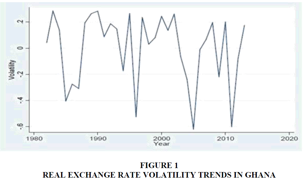
Figure 1: Real Exchange Rate Volatility Trends In Ghana
Furthermore, the coordinated development programmes such as the Ghana Poverty Reduction Strategy (GPRS I, 2003-2007), Growth and Poverty Reduction Strategy II (GPRS II, 2006-2009), Ghana Shared Growth and Development Agenda (GSGDA I, 2010-2013) & GSGDA II (2014-2017) which were meant to ensure stable macro-economy and financial market, have not lived up to their desired expectations. Currently, the medium-term development policy framework which is also a coordinated programme under the name Agenda for Jobs (MTDPF, 2018-2021) is under implementation to provide policies and strategies that can also help in maintaining a stable a stable economy. Against this background, we posit that, Ghana is still bedevilled with exchange rate fluctuations and hence the need to further investigates its effects on economic growth.
Methodology
Data
With 36 observations (time series data spanning from 1980 to 2015), data on all variables except political dummy and exchange rate dummy are sourced from the World Development Indicators (WDI) dataset. Political and exchange rate regime dummies were constructed by the authors using historical evidence. We posit that, all else held constant (i.e. traditional domestic growth determinants), REER negatively impacts on Ghana’s growth prospects. In line with Solow (1956) and later Mankiw et al. (1992) who acknowledge that physical and human capital are complementary factors of economic growth, we define our traditional growth model as:
Yt = Af(Kt Lt)
Where, Y is the level of output or economic growth which is measured as GDP per person growth rate. It depends on some units of physical capital (K) and human capital or labor (L), while t denotes time period in years. Next, we specify an augmented growth accounting model that incorporates REER volatility (Vt) and additional control variables represented as vector Z. A similar approach where a growth model was tweaked to incorporate new variables can be found in De Mello (1999), Borensztein et al. (1998), Acikgoz et al. (2016) and Awad & Ragab (2017). This is presented as:
Yt = (Kt LtVt Zt)
Above equation is re-specified empirically for estimation purposes and presented below as:

Dependent Variable: Y
GDP per person growth rate (Yt) in above equation, is constructed using the difference between the GDP per capita (constant 2010) at time, t (gdppct) and time, t lag 1 (gdppct−1), divided by the latter and multiplied by 100. This is considered as an appropriate measure of a country’s growth rate because measures the rate of growth in the value added or the final goods and services produced per person of a country over a period of time. One would expect more injections to trigger more economic or productive activities which in effect increase the level of output growth per person. On the other hand, one would expect any leakage to hurt economic growth prospects hence a negative relationship with economic growth.
Independent Variables
Using, REER as a measure of instability in commodity trade at the international level. Given the short-comings in the use of standard deviations (Gadanecz & Mehrotra, 2013) as a measure of volatility, we used the Autoregressive Conditional Heteroscedasticity (ARCH) and Generalized ARCH (GARCH) to measure the degree to volatility. Thus, we used the GARCH (1, 1) to determine the conditional variance. We follow the specification by Oseni (2016) to obtain the conditional variance of the REER. First, we specify mean equation as follows:
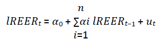
Where, lREERt and lREERt−1 are the log of the REER and the log of the lag of the REER respectively, with as our error term. Next, we obtained the conditional variance equation as:
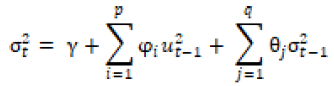
Where, σ2t and σt-1 and  are the volatility, the lag of the volatility (GARCH term) and the ARCH term respectively. The volatility obtained is plugged into re-specified equation, to firstly estimate the effect of real exchange rate volatility on economic growth using a simple regression equation. For robustness of results, four more models are estimated with controls. Second, we generate an index of financial performance fragility by interacting three different measures of financial market development. In generating the interactive term, we selected five measures that are very relevant to sub-Saharan Africa. This includes a measure of bank performance (market capitalization), asset quality (non-performing loans), managerial efficiency (cost to revenue ratio), and financial fragility (z-score). We undertook a Principal Component Analysis (PCA) and selected two measures based on their eigen values. A third variable (z-score) which provides a measure of financial fragility was added to yield a third term to generate the interaction term. See Appendix 1 for the PCA results. This interaction term was generated to further investigate whether REER volatility still hurts economic growth after controlling for financial market fragility.
Human capital and physical capital are both considered as traditional variables that explains a country’s level of economic activities. As a proxy for human capital, we used the share of labour force to the total population which is a labour-market characteristic. Given the paucity of human capital variables for the country understudy, this proxy better represents the number of workers in the population or the number of workforce in the population. Also, our dataset is challenged by some missing data. This was augmented by using five-year moving averages. It is worth mentioning that even estimating the model without the moving averages still showed some robustness. Thus, the sign and significance of all variables remained unchanged. However, the number of observations and the magnitude of the coefficients changed marginally. Labour which is a human capital plays a key role in explaining the economic growth. All else held constant, an increase in the labour force is expected to have a positive effect on GDP per capita growth.
Additionally, developing countries such as Ghana rely heavily on developed countries for capital inputs. Against this background, we argue that it will not be out of place to use FDI as a proxy for capital. All other things being equal, we expect capital to vary positively with GDP per capita growth.
Also, we included inflation in our model to control for possible market uncertainties or macroeconomic instability which is a common feature in developing countries. These macroeconomic policy variables are deemed critical in macroeconomic models of this nature. We expect inflation to vary negatively with GDP per capita growth.
Again, “R” is captured as a dummy in re-specified equation to represent various exchange rate regimes (i.e. Zero (0) for periods of fixed exchange rate; and one (1) for periods of full flexible exchange rate regimes).
Also, “P” is included in the model as a dummy for political regimes. Here we have zero (0) for periods where the country was governed by military government and one (1) for periods of democratic rule.
Lastly, given that markets in Africa are open, small and fragile because they are mostly susceptible to shocks from developed economies; we introduced a variable to control for possible fragility in Ghana’s financial market. We controlled for possible fragility in Ghana’s financial market using the fragility indices as developed by Andrianova et al. (2015). We interacted three of the indices (i.e. z-score, equity and return on assets) that are expected to have a positive coefficient on GDP per capita growth.
Table 1 shows the descriptive statistics of all variables used in our model for the estimation. The mean of the GDP per capita growth rate is 1.77% with a minimum value of -9.93%, a maximum value of 11.28% and a standard deviation of approximately 3.73%. This shows a moderately high spread.
| Table 1 Descriptive Summary Statistics |
||||||||
| Stats | Y | INF | REER-Volatility | LAB | FDI | Fragility | P | R |
| Mean | 1.77 | 30.75 | 1.404755 | 0.73 | 2.91856 | 412.6676 | 0.64 | 0.33 |
| Median | 1.95 | 25.02 | .0906981 | 0.72 | 1.66393 | 431.3845 | 1.00 | 0.00 |
| Standard dev | 3.73 | 22.40 | 3.300405 | 0.189 | 3.21032 | 147.0889 | 0.48 | 0.48 |
| Skewness | -1.04 | 2.48 | 2.796022 | 0.51 | 0.94327 | 1.106041 | -0.58 | 0.71 |
| Kurtosis | 6.22 | 9.81 | 10.0366 | 3.42 | 2.34329 | 6.310542 | 1.33 | 1.5 |
| Min | -9.93 | 11.15 | .0042598 | 0.69 | 0.04533 | 121.6386 | 0 | 0 |
| Max | 11.28 | 123.06 | 14.55152 | 0.77 | 9.51704 | 890.4134 | 1 | 1 |
| N | 36 | 36 | 36 | 36 | 36 | 36 | 36 | 36 |
Note: P and R are political and exchange rate regimes respectively.
The real effective exchange rate volatility shows enough evidence of volatility with a mean of 1.41% and a higher standard deviation of 3.30%. The inflation rate which shows the rate of uncertainty in the market prices provides a high spread with a mean of 30.8% but a standard deviation of 22.4%. Also, FDI shows evidence of high variability with a mean of 2.9% and a standard deviation of 3.2%. Similarly, fragility in the financial market provides a distribution that is not normal with higher tails in the distribution as evidenced by the skewness and the kurtosis. On the contrary, labour shows a distribution that is near normal, given that the measures of central tendency are quite close, with skewness of almost zero and kurtosis of approximately 3. Since 1980, the political dummy (P) variable shows that Ghana has averagely enjoyed more democratic rule as compared to military rule. For exchange rate regime dummy, we have evidence that periods of fully market determined flexible exchange rate is averagely less than periods of an alternative exchange rate.
Estimation Strategy
According to the Gauss-Markov theorem, the estimated coefficients of an Ordinary Least Squares (OLS) model is described as the Best Linear Unbiased Estimator F (BLUE) provided the errors have expectation zero and are uncorrelated and have equal variances. In many cases, the means and the variances do change over time which violates the assumption and results in spurious regression (i.e., when time series data exhibit non-stationary tendencies). The procedure for testing the presence or otherwise of the unit root of a series in a general time series setting is very critical. In this study, we apply both Augmented Dickey-Fuller (ADF) and Dickey Fuller-GLS (DF-GLS) stationary tests. The results are presented in Table 2.
| Table 2 Stationarity Test |
||||
| Augmented Dickey fuller(ADF) | Phillips-Perron(PP) | |||
| Variable | Test statistic | Test statistic | ||
| Constant | Constant and trend | Constant | Constant and trend | |
| Reer-vol | -3.441*** | -3.169* | -2.177 | -2.926 |
| d.reer-vol | -6.834*** | -9.769*** | -5.601*** | -5.506 *** |
| Y | -4.935*** | -5.331*** | -2.659* | -3.954591*** |
| dY | -4.024*** | -3.983 *** | -7.293 *** | -3.400** |
| Fragility | -4.320*** | -4.899079*** | -4.911206*** | -5.044310*** |
| dFragility | -4.886*** | -7.752509*** | -7.994038*** | -7.542 *** |
| fdi | -0.523 | -2.255 | -0.605 | -2.318 |
| dfdi | -3.336*** | -3.374** | -4.908*** | -4.883*** |
| lab | -3.272** | -3.644** | -1.119 | -1.425 |
| dlab | -3.741*** | -3.758*** | -5.644†*** | -5.554†*** |
| inf | -4.586 *** | -4.752 *** | -4.752*** | -6.472*** |
| dinf | -4.755 *** | -4.810*** | -15.861*** | -16.029*** |
Note: Null Hypothesis: D (Y, 0, 1) has a unit root; †D (L, 2) has a unit root ***p<0.01, **p<0.05, *p<0.1.
With the null hypothesis of unit root (non-stationarity), if the p-value is less than five percent, we reject the null hypothesis and conclude that the series are stationary. In contrast, if the p-value is greater than five percent, we accept the null hypothesis and proceed with first differencing, else the regression results will be deemed spurious. We have evidence from the ADF results that all five out of six series have unit root at 1% and 5% levels of significance respectively. However, with the exception of only three variables (reer_vol, lab and fdi), all variables under PP were stationary at levels. This suggests that most of the series are stationary even at levels. That notwithstanding, we differenced all the series and can argue that the series are without unit root. Based on the ADF test, we conclude that the time series variables used in our study are I (0) & I (1) variables. Thus, we have evidence that our time series variables are stationary, so long-run coefficients cannot be spurious. That notwithstanding, given that our econometric technique is characterized by an instrumental variable estimator that provides robust estimators for both stationarity and non-stationarity variables, we proceed with the test for long-run equilibrium (Kwablah et al., 2014).
Test for Long-run Equilibrium
This study uses the Johansen co-integrating equation to determine the long-run equilibrium relationships among the set of variables. From the Trace and Maximum-Eigen values, we have evidence of at least two co-integrating equations irrespective of the choice of model presented in Table 3.
| Table 3 Johansen Co-Integration Test |
|||||
| Data Trend: | None | None | Linear | Linear | Quadratic |
| Test Type | No Intercept | Intercept | Intercept | Intercept | Intercept |
| No Trend | No Trend | No Trend | Trend | Trend | |
| Trace | 3 | 3 | 3 | 4 | 4 |
| Max-Eig | 2 | 3 | 3 | 4 | 4 |
Note: Critical and probability values based on MacKinnon et al. (1999).
Selected (0.05 level*) No. of Cointegrating Relations by Model. Lags interval: 1 to 2
Econometric Technique
We now turn our attention to applying the Fully Modified Ordinary Least Squares (FMOLS) as our econometric technique to estimate and investigate whether exchange rate volatility is still deleterious to growth after controlling for fragility in the financial market. We admit that OLS may not be appropriate for studies of this nature because of identification issues such as serial correlation, endogeneity, heteroscedasticity etc. We resort to the FMOLS econometric technique. The FMOLS provides some modifications to the traditional OLS technique and makes standard asymptotic inference plausible. Thus, making them asymptotically equivalent (Phillips, 1995; Kwablah et al., 2014). The FMOLS is a single equation estimator for co-integrated relationships. This dynamic estimator was first developed by Phillips and Hansen (1990) to use a semi-parametric strategy in dealing with issues of endogeneity and serial correlation commonly associated with long-run estimations. In the absence of co-integration among the regressor’s and large samples, this robust econometric technique still provides consistent and efficient estimates. We follow Kwablah et al. (2014), and present the standard time series FMOLS estimator as:
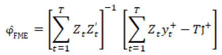
Where the correction is term for endogeneity and
  is the serial correlation term.
We present a pairwise correlation matrix in Table 4 which shows the extent to which all variables used in the FMOLS econometric model are correlated. Generally, pairwise correlation test shows the following: correlation coefficient, probability values and the number of observations. The lowest and highest correlation coefficients are given as approximately 0.005 and 0.65 respectively. We used p value of 1% and conclude that although there is evidence of correlation among some of the variables, it is not severe to influence our variances and co-variances and as such the precision of our estimation.
| Table 4 Correlation Matrix Of Covariates |
|||||||
| VARIABLES | REER_VOL | FDI | INF | LAB | FRAGILITY | P | R |
| REER_VOL | 1 | ||||||
| P-value | N/A | ||||||
| Obs | 36 | ||||||
| FDI | -0.3644 | 1 | |||||
| P-value | 0.0289 | N/A | |||||
| Obs | 36 | 36 | |||||
| INF | 0.4757 | -0.3855 | 1 | ||||
| P-value | 0.0034 | 0.0202 | N/A | ||||
| Obs | 36 | 36 | 36 | ||||
| LAB | -0.1585 | 0.4630 | -0.3174 | 1 | |||
| P-value | 0.3559 | 0.0045 | 0.0593 | N/A | |||
| Obs | 36 | 36 | 36 | 36 | |||
| FRAGILITY | 0.0779 | -0.250421 | 0.00462 | 0.0691 | 1 | ||
| P-value | 0.6516 | 0.1407 | 0.789 | 0.6889 | N/A | ||
| Obs | 36 | 36 | 36 | 36 | 36 | ||
| P | -0.5544 | 0.6416 | -0.3637 | 0.2999 | -0.1261 | 1 | |
| P-value | 0.0005 | 0 | 0.0292 | 0.0755 | 0.4637 | N/A | |
| Obs | 36 | 36 | 36 | 36 | 36 | 36 | |
| R | 0.5849 | -0.6059 | 0.4229 | -0.2801 | 0.1266 | -0.6450 | 1 |
| P-value | 0.0002 | 0.0001 | 0.0102 | 0.098 | 0.4618 | 0.0000 | N/A |
| Obs | 36 | 36 | 36 | 36 | 36 | 36 | 36 |
Structural Break Test
Considering the fact that the economy of Ghana has witnessed different political and exchange rate regimes, it is imperative to examine the possibility of such regimes on the sample dataset. We admit that using Quandt-Andrews breakpoint test will not be ideal as it will affect our data points. So, we used the Chow breakpoint test which is a more specific to the year of the transition (i.e. 1992). The results presented (Appendix 1), provides evidence that we cannot reject the null hypothesis of no significant structural break in 1992. We can therefore proceed with the estimation.
Results And Discussion
In this section, we present the findings and analysis of the results from the stationarity, co-integration and the long run economic growth elasticity’s as a result of the role of exchange rate volatility and control covariates.
Table 5 shows the regression results of five estimated models. In all, we run a regression of GDP per person growth rate on exchange rate volatility with and without controls, using the FMOLS technique. We find that exchange rate volatility is negative and statistically significant across all estimated models. Thus, as expected, we have evidence from all the estimated models that exchange rate volatility is very harmful to economic growth prospects. It is mainly possible through the channels of investment and consumption expenditures. We justify our results by arguing that during periods of high fluctuations in the real exchange rate; foreign trade, investments, capital movements, international trade and economic growth are affected negatively. Given model 5 as our final model, we find that a 1% increase in real exchange rate volatility decreases GDP per person growth rate by approximately 0.19%. Thus, we argue that lack of stability in the foreign exchange market does not augur well for Ghana’s economic growth prospects. Our finding is in line with Dollar (1992), and more recently Alagidede & Ibrahim (2017). These studies have both shown that volatility and depreciation are inimical to economic growth performance. However, stabilizing real exchange rate can spur growth performance in developing countries.
| Table 5 Regression Results |
|||||
| Variables | (1) | (2) | (3) | (4) | (5) |
| FMOLS | FMOLS | FMOLS | FMOLS | FMOLS | |
| Real Exchange rate volatility | -0.6029*** | -0.3219* | -0.2265*** | -0.2147*** | -0.1924*** |
| (0.164) | (0.172) | (0.069) | (0.058) | (0.029) | |
| Inflation | -0.0790*** | -0.0571*** | -0.0611*** | -0.0620*** | |
| (0.027) | (0.011) | (0.009) | (0.004) | ||
| Foreign Direct Investment | 0.3403*** | 0.3868*** | 0.3780*** | ||
| (0.070) | (0.065) | (0.034) | |||
| Labour Force | -24.4316** | -30.5997*** | |||
| (10.330) | (4.637) | ||||
| Financial Fragility | 0.0026*** | ||||
| (c.zr#c.equity#c.roaa) | (0.001) | ||||
| political dummy | 1.6686*** | ||||
| (0.476) | |||||
| Exchange Rate Regimes | 1.2988*** | ||||
| (0.484) | |||||
| Constant | 2.7281*** | 4.7247*** | 2.8053*** | 20.5512*** | 22.5587*** |
| (0.615) | (0.890) | (0.466) | (7.491) | (3.328) | |
| Observations | 35 | 35 | 35 | 35 | 35 |
| R-squared | 0.020 | 0.318 | 0.322 | 0.307 | 0.207 |
| Bandwidth(newey-west) | 2.9529 | 49.3416 | 29.4725 | 28.6551 | 64.0250 |
Note: Dep Variables: Y (Gross Domestic Product per person Growth Rate);
Standard errors in parentheses ***p<0.01, **p<0.05, *p<0.1
In this study, we used inward FDI as a proxy for capital or better still physical factor endowment commonly found in growth models. Gross capital formation is not used in this study given that:
The quality of government and households fixed capital formation tends to be weak in most developing countries. We are interested in a variable that shows new capital investments. So, concerning the new growth theory, Awad & Ragab (2017) used FDI to represent an additional source of capital injection from the source country to the host country. It was used under the assumption that developing countries depend on FDI for an increase in physical capital. We find positive and highly statistically significant coefficients for all the estimated models. From our final model 4, we have evidence that a 1% increase in FDI increases GDP per person growth rate by about 0.50%. It is in line with findings from earlier studies such as Awad & Ragab (2017), Elkomy et al. (2016) and Ahiabor & Amoah (2013).
Again, we measured human capital with the share of active labour force to the total population. A priori, we were expecting an increase in labour force to have a positive effect on growth. Interestingly, within the period understudy, we found a negative relationship between human capital and GDP per person growth. This finding is plausible for the fact that illiteracy rate in Ghana is high. This has resulted in the supply of low quality and unskilled labour to the market. In effect, this adds to cost because of low productivity. Obviously, such low quality unskilled labour will definitely be associated with low wages and salaries. Thus, higher fraction of labour force being unskilled will not be without its negative repercussion on GDP per person growth. To help address this challenge, the government of Ghana in 2017 rolled out the Free Senior High School policy to help reduce the supply of unskilled labour to the labour market.
We controlled for possible market uncertainties (macroeconomic instability) with the general price level, inflation. The Friedman-Ball hypothesis and Cukierman-Meltzer hypothesis have posited that higher rates of inflation cause inflation volatility (Barimah & Amuahkwah, 2012). Also, empirically (Jha & Dang, 2011), we have found some evidence that inflation volatility is deleterious to economic growth, especially for developing countries. Similar to existing empirical findings, with a highly statistically significant probability value, we find that a 1% increase in inflation decreases GDP per person growth rate by 0.06%. Thus, we have evidence that market uncertainties hurt economic growth in Ghana.
Again, we controlled for the possible influence of various exchange rate regimes on economic growth. We found that periods of flexible exchange rate are associated with an increase in economic growth rates. Thus, we have highly statistically significant evidence that the probability of having a flexible exchange rate relative to fixed exchange rate increases GDP per person growth rate by approximately 1.30%. It is in line with our expected results, in that, empirical evidence (Alba et al., 2010) has shown that Foreign Direct Investment (FDI) which intuitively varies positively with growth, rises with the flexible exchange rate. Hence one would expect that, in the case of Ghana, the GDP per person growth rate rises under flexible exchange rate regimes compared to fixed exchange regimes in Ghana.
Again, we controlled for the different political regimes experienced within the period of the study. We have evidence that periods of democratic rule positively impact on GDP per person growth rate relative to periods of military rule. Thus, in Ghana, wellbeing of the people has improved under democratic rule than the military rule.
Again, one factor that influences the way exchange rate fluctuations affect economic growth is the development level of financial markets. So we controlled for this using a new measure of financial market development that accounts for fragility, we found a positive and significant relationship as expected. Thus, an increase in the fragility indices implies less vulnerability in Ghana’s financial market yielding an increase in economic growth (Mensah et al., 2016). On the other hand, a more fragile financial market is also inimical to economic growth in Ghana.
Conclusion
Empirical evidence on the relationship between exchange rate volatility and economic growth with welfare implications has been inconclusive in the literature. This study sought to expand this empirical discourse especially for a developing country like Ghana which has in recent times experienced serious financial market challenges (Asiama & Amoah, 2018). It is important to acknowledge that, this is not the first study to investigate this relationship. A key point of departure from previous studies is the fact that we accounted for financial market fragility which is critical given the recent happenings in Ghana’s financial sector.
The first objective of this paper was to investigate whether real exchange rate volatility hurts economic growth in Ghana. In addition, given the fragile nature of Ghana’s financial sector, we investigated whether after accounting for financial market fragility, real exchange rate volatility will still hurt economic growth. We used annual time series data from 1980-2015. Applying the FMOLS econometric technique as a way of dealing with endogeneity and serial correlation issues, we estimated four models with and without controls. Generally, the models that did not account for financial market fragility were consistent in sign and in significance with the model that accounted for it. In all, we have evidence that real exchange rate volatility varies negatively with economic growth in Ghana. This is plausible given that, for an import dependent and highly unprocessed traditional export country like Ghana, fluctuation in the exchange rate results in a relatively weaker domestic currency which makes it susceptible to excessive imports over exports. The net import of the country which is a leakage ends up hurting domestic country’s growth. This finding is consistent with results by Alagidede & Ibrahim (2017), Ndambendia & Alhayky (2011); Aghion et al. (2009); Bagella et al. (2006) among others as earlier reviewed. However, Aliyu (2009) and Adeniran et al. (2014) had contradictory results which could be attributed to identification strategy challenges which were not properly addressed in their papers. For example, Aliyu (2009) acknowledged possible reverse causality between the variables of interest, yet this was not addressed in the paper. Also, Adeniran et al. (2014) applied OLS on a time series data and failed to account for possible serial correlation and endogeneity issues. By this, one can conclude that their results may be driven by identification issues. Another reason for the positive effect of volatility in exchange rate could be attributed to country unique macroeconomic differences. In Nigeria, for example, competitiveness in oil and foreign exchange market may perhaps be the driving force for such positive results. We posit that most studies that have had consistent results with ours mainly employed econometric techniques that sought to address such identification challenges.
This study recommends that measures should be put in place to build Ghana’s international competitiveness in trade. This will help improve Ghana’s trade balance, increase forex reserves, and reduce demand for foreign exchange to finance import of capital goods and technology. This will help strengthen the local currency and stabilize the fluctuations, which may end up reducing the excessive fluctuation in the exchange rate. This is possible if the country diversifies its trade and desists from over-relying on traditional exports for foreign exchange generation. Thus, harnessing the opportunities in non-traditional exports should be considered. In addition, managers of Ghana’s economy should focus on strengthening the macroeconomic fundamentals which is critical for stabilizing the market based flexible exchange rate.
References
- Acikgoz, B., Amoah, A., & Yılmazer, M. (2016). Economic freedom and growth: A panel cointegration approach. Panoeconomicus, 63(5), 541-562.
- Adeniran, J.O., Yusuf, S.A., & Adeyemi, O.A. (2014). The impact of exchange rate fluctuation on the Nigerian economic growth: An empirical investigation. International Journal of Academic Research in Business and Social Sciences, 4(8), 224.
- Adu-Gyamfi, A. (2011). Assessing the impact of exchange rate volatility on economic growth in Ghana.
- Aghion, P., Bacchetta, P., Ranciere, R., & Rogoff, K. (2009). Exchange rate volatility and productivity growth: The role of financial development. Journal of Monetary Economics, 56(4), 494-513.
- Ahiabor, G., & Amoah, A. (2013). The Effects of Corporate Taxes on the level of Investment in Ghana. Development Country Studies, 3(1), 57-67.
- Alagidede, P., & Ibrahim, M. (2017). On the causes and effects of exchange rate volatility on economic growth: Evidence from Ghana. Journal of African Business, 18(2), 169-193.
- Alba, J.D., Wang, P., & Park, D. (2010). The impact of exchange rate on FDI and the interdependence of FDI over time. The Singapore Economic Review, 55(04), 733-747.
- Aliyu, S.U.R. (2009). Impact of oil price shock and exchange rate volatility on economic growth in Nigeria: An empirical investigation.
- Andrianova, S., Baltagi, B., Beck, T., Demetriades, P., Fielding, D., Hall, S., Koch, S., Lensink, R., Rewilak, J., & Rousseau, P. (2015). A new international database on financial fragility. University of Leicester Economics Working Paper, 15, 18.
- Asiama, R.K., & Amoah, A. (2018). Non-performing loans and monetary policy dynamics in Ghana. African Journal of Economic and Management Studies.
- Awad, A., & Ragab, H. (2018). The economic growth and foreign direct investment nexus: Does democracy matter? Evidence from African countries. Thunderbird International Business Review, 60(4), 565-575.
- Baba, I., & Bangniyel, P. (2014). The dynamics of real exchange rate volatility and economic growth in a small open economy. Researchjournali’s Journal of Finance, 2(8), 2-9.
- Bagella, M., Becchetti, L., & Hasan, I. (2006). Real effective exchange rate volatility and growth: A framework to measure advantages of flexibility vs. costs of volatility. Journal of Banking & Finance, 30(4), 1149-1169.
- Barimah, A., & Amuakwa-Mensah, F. (2014). Does inflation uncertainty decrease with Inflation? A GARCH model of inflation and inflation uncertainty for Ghana. Journal of Monetary and Economic Integration, 12(2), 32-61.
- Bleaney, M., & Greenaway, D. (2001). The impact of terms of trade and real exchange rate volatility on investment and growth in sub-Saharan Africa. Journal of Development Economics, 65(2), 491-500.
- Borensztein, E., De Gregorio, J., & Lee, J. W. (1998). How does foreign direct investment affect economic growth? Journal of international Economics, 45(1), 115-135.
- De Mello, L.R. (1999). Foreign direct investment-led growth: Evidence from time series and panel data. Oxford Economic Papers, 51(1), 133-151.
- Dollar, D. (1992). Outward-oriented developing economies really do grow more rapidly: Evidence from 95 LDCs, 1976-1985. Economic Development and Cultural Change, 40(3), 523-544.
- Elkomy, S., Ingham, H., & Read, R. (2016). Economic and political determinants of the effects of FDI on growth in transition and developing countries. Thunderbird International Business Review, 58, 347-362.
- Gadanecz, B., & Mehrotra, A. (2013). The exchange rate, real economy and financial markets.
- Jha, R., & Dang, T. N. (2012). Inflation variability and the relationship between inflation and growth. Macroeconomics and Finance in Emerging Market Economies, 5(1), 3-17.
- Kwablah, E., Amoah, A., & Panin, A. (2014). The impact of foreign aid on national income in Ghana: a test for long-run equilibrium. African Journal of Economic and Sustainable Development, 3(3), 215-236.
- MacKinnon, J.G., Haug, A.A., & Michelis, L. (1999). Numerical distribution functions of likelihood ratio tests for cointegration. Journal of Applied Econometrics, 14(4), 563-577.
- Mankiw, N.G., Romer, D., & Weil, D.N. (1992). A contribution to the empirics of economic growth. The Quarterly Journal of Economics, 107(2), 407-437.
- McKinnon, R.I. (1963). Optimum currency areas. The American Economic Review, 53(4), 717-725.
- Mensah, J.T., Adu, G., Amoah, A., Abrokwa, K.K., & Adu, J. (2016). What drives structural transformation in sub-Saharan Africa? African Development Review, 28(2), 157-169.
- Ndambendia, H., & Alhayky, A. (2011). Effective real exchange rate volatility and economic growth in sub-Saharan Africa: evidence from panel unit root and cointegration tests, The IUP Journal of Applied Finance, 17(1), 85-94.
- Oseni, I.O. (2016). Exchange rate volatility and private consumption in Sub-Saharan African countries: A system-GMM dynamic panel analysis. Future Business Journal, 2(2), 103-115.
- Phillips, P.C.B. (1995). Fully modified least squares and vector autoregression. Econometrica: Journal of the Econometric Society, 63 (5), 1023-1078.
- Phillips, P.C.B., & Hansen, B.E. (1990) ‘Statistical inference in instrumental variables regression. Journal of Economics, 70(1), 65-94.
- Solow, R.M. (1956). A contribution to the theory of economic growth. The Quarterly Journal of Economics, 70(1), 65-94.
- Yeboah, O., Shaik, S., & Quaicoe, O. (2012). Evaluating the causes of rising food prices in low and middle income countries. Journal of Agricultural and Applied Economics, 44(3), 411-422.