Keywords

GST, GTMA, Macroeconomics, Taxation, Government Revenue, Macroeconomic Stabilization

Introduction

What is GST?

GST, also known as Goods and Service Tax, passed in the Lok Sabha on 29^th March 2017 and came into effect from 1^st July 2017 under the GST Act or Constitution (One Hundred and First Amendment) Act, 2016. The tax went into the picture as another type of indirect tax, which is a levy in place of previous existing taxes. The idea behind the introduction of is to have GST replaced an array of indirect taxes under a unified tax regime and is thus is expected to reshape the country's economy anew.

History of GST

The L K Jha committee was foremost dyed the need to turn into the Value Added Tax regime (VAT) in India, 1974. Chelliah committee proposed VAT or GST execution in 1991. Service Tax executed in India, 1994. In 2000, the Vajpayee Government started the discussions on GST, by setting up an empowered committee, headed by Asim Dasgupta, the then Finance Minister, Government of West Bengal. The committee assigned the task of designing the GST model and overseeing the IT backend preparedness for its rollout. Moving towards GST was then again reflected by, then, Union Finance Minister in his Budget discourse for 2006-07. At first, it was recommended that GST would be presented from first April 2010. The Empowered Committee of State Finance Ministers (EC), which had figured the outline of State VAT was asked to create a guide and structure for GST for altering according to the need of everyone to be catered. Joint Working Groups of authorities having agents of the States and additionally the center were set up to inspect different parts of GST and draw up reports particularly on exclusions and edges, tax collection of administrations and tax assessment of between State supplies in accordance to fulfill the role in removing excess taxes on multi-level stages. In light of dialogs inside and amongst it and the Central Government, the EC discharged its First Discussion Paper (FDP) on the GST in November 2009. The FDP released in November 2009 beckons out highlights of the proposed GST and had framed the reason for exchange between the Centre and the States up until recent. The Goods and Services Tax (GST) is a novel idea that simplifies the complex tax structure by supporting and enhancing the economic growth of a country. GST is an extensive tax levy on the manufacturing, sale, and consumption of goods and services at a national level Dani (2016).

The Goods and Services Tax Bill or GST Bill, also referred to as The Constitution (One Hundred and Twenty-Second Amendment) Bill, 2014, initiates a Value-added Tax to be implemented on a national level in India. GST will be an indirect tax at all the stages of production to bring about uniformity in the system. On bringing GST into practice, there would be an amalgamation of Central and State taxes into a single tax payment. It would also enhance the position of India in both domestic as well as international market. At the consumer level, GST would reduce the overall tax burden, which is the current estimate at 25-30% Dani (2016). Under this system, the consumer pays the final tax, but an efficient input tax credit system ensures that there is no cascading of taxes- a tax on tax paid on inputs that go into the manufacture of goods. To avoid the payment of multiple taxes such as excise duty and service tax at the Central level and VAT at the State level, GST would unify these taxes and create a uniform market throughout the country. The integration of various taxes into a GST system will bring about an effective cross-utilization of credits. The current system taxes production, whereas the GST will aim to tax consumption. Experts have enlisted the benefits of GST as under:

1. It would introduce a two-tiered One-Country-One-Tax regime.

2. It would subsume all indirect taxes at the center and the state level.

3. It would not only widen the tax regime by covering goods and services but also make it transparent.

4. It would free the manufacturing sector from the cascading effect of taxes, thus improving the cost-competitiveness of goods and services.

5. It would bring down the prices of goods and services and, thus, increase consumption.

6. It would create a business-friendly environment, thus by increase the tax-GDP ratio.

7. It would enhance the ease of doing business in India.

8. Some of the best GST systems across the world like Singapore and New Zealand use single GST, but India has opted for a dual GST model Dani (2016) &Venkatesh (2015) The change in tax structure is expected to have a significant impact on the supply chain in India. A comparison of the GST rates of some countries with the proposed India GST rate is mentioned in Table 1 Venkatesh (2015).

Table 1 Rates of Taxes Levied in Different Countries
Country	The rate of GST (%)
Australia	10
Canada	5
New Zealand	15
Singapore	7
Malaysia	6
Sweden	25
India	27*

Literature Review

GST as a tax structure can be loosely defined as the amalgamation of several centers and state-driven taxes into a single umbrella of the GST tax regime. The primary driving factor for an introduction to GST has created an even market for making tax structure easier at domestic level and international investment favourable environment for tax-driven Indian Economy. At the consumer level, GST would reduce the overall tax burden, which is currently estimated at 25-30% Dani (2016). In the face to create tax structure unified and straightforward to reduce the problems of payments of a different centre run and state-run taxes at different levels of the supply chain, it dissolves in all the taxes into a single one to create an unformalized market with easier access. While it has been noted that most of the tax will be burdened over the end-user and consumers, but GST still holds the claim to reduce total tax burdens by margins. However, the devised bill may have been drafted with the idea to ease in the current economy and create a tax-friendly market for the producers. The idea of ease of understanding and to uniform the tax structure can be structured on various factors and parameters like ease of application of tax, both at corporate and individual level, and reducing the confusion at various levels of taxation, which may also lead to tax evasions as well. There still can be several factors on which it can be measured by its performances over the term of implementations, which can be significantly varied with high correlation to each other and while some may be entirely independent of each other. This type of approach to determine the performance a particular strategy on selected varied factors requires checking the performance of the observed scenarios by each factor independently and simultaneously at a level dependent on one another. This type of evaluation can give hidden information about the structure which can be much clouded on the terms of factors when seen as a whole. The method described also gives the picture of the nature of planning during the stages of the drafting of such strategic steps and the agenda of the implementation body about the type of problems it was tailored for, both at bureaucratic and corporate levels. The bill can be further tested by satisfaction of individuals towards its implementation Moorman et al. (1993). Here the different dispositions of different factors and attributes are being observed by the satisfaction index to find the overall performance of the cases in different aspects of the uniformity and prospects of future elevation. The three scenarios that have been studied in this case are current implementation and its implementation period, Post-Demonetisation period and one of the hypothetical cases if the GST would have been introduced following demonetization simultaneously. The prior two cases are real-world instances and in their accordance, while the latter one is hypothetical, which aims to find the robustness of GST as a bill for Indian domestic and international markets in cases of sharp blows. The three given disposition alternatives are chosen and are then tested for their implementations on the specific factors. The three cases are introduced in brief below.

Current Implementation or Post-GST Period

The case illustrates the period after the successful implementation of GST in India. The basis of comparison is the Pre-GST period with the conventional tax-regime that was present in India. The Lok Sabha passed the Bills on 29^th March 2017. The Rajya Sabha passed these Bills on 6^th April 2017 and was then enacted as Acts on 12^th April 2017. For the sake of convenience, the case is referred to as Post-GST period later in the paper.

Post-Demonetisation Period

This case illustrates the condition of domestic Indian markets and trade in the period after the demonetization was implemented on the existing currency notes by then Prime Minister Narendra Singh Modi. The announcement of demonetization was made on 8^th November 2016 with the effect of denouncing all high currency notes of ₹1000 and ₹500 and getting new currency notes of ₹2000 and ₹500 in circulation in hope to curb the black money and counterfeit currency.

Post-Demonetisation period with successively implemented GST (Hypothetical)

This case is taken hypothetically for the instance if the GST has happened after just weeks to demonetization. The primary aim of this case is to check the robustness of the drafted bill and for the understanding its validation in case of any such unexpected future occurrences to float out the country’s economy with the least citizen discomfort.

The process of selection for the cases mentioned above and alternatives can vary according to the observer, but the main reason for choosing the above-specified alternatives for the selection can be mainly attributed to the fact them being the most highlighted events in the Indian economy in recent periods. The focus of the project is on the application of GST and its performance measure for the soundest effect of it on the then Indian markets and with more considerable implications on the current and future trade of the domestic and foreign market affairs. The second case of the Demonetisation was taken into consideration with the fact that India observed a significant slowdown after the implementation in the financial year 2017. This case works as a precise scale for any of the unexpected slowdowns that may occur in the future to provide a reference. Some of the ramifications of the same can be said to be rippled during the global slowdown in late 2019 global economic slowdown as India continues to face declining GDP growth. The factors on which the above cases are grounded upon and are compared their performance against are mainly inclined towards the ease of working in Indian markets while others are in conjugation to the performance of the economy. While the significant setbacks were visible on the comfort of the citizens as cited by all major news outlets, the effects of the demonetization on the market and trade affairs remain unclear, with many of the economists and finance experts divided on their views. The last case is a hypothetical one where the GST introduced in the period of the near demonetization implementations. While the GST bill was introduced in early July 2017 to be efficiently implemented in the markets, the case of demonetization has already been in vain with its significant impacts already delivered to the Indian markets. Thus it has been assumed that if the GST was successfully implemented in the markets in the period of late November or early December 2016. The primary purpose of the case is to find out the performance of GST in the cases of uncertainties and precipitous effects of specific instances.

The GST bill is being scaled for the robustness on the basis that whether it can help as a deterrent for the future instances where any uncertain event with large-scale implications can be withstood or if the structure of Indian economy and taxes become more brittle and vulnerable. The main objective of the study is found to observe the GST as a bill for the stability of Indian domestic and foreign markets. Pierre J. Richard et al. (2009) developed methods to calculate the organizational performance using multi-dimensional conceptualization Agrawal et al. (2016). Used the methods of GTMA for the analysis of different alternatives and their feasibility on the scale of specific features for the topic of reverse logistics.

Methodology

The comparison is performed on different levels of influence subjected to the discussed factors by their inclusivity on the drafting of the act. The draft in itself is devised on some factors which are to be concerned for significant welfare on the scale for the majority of the populace and future aspect of amendment and execution ability. The approach towards the comparison of these different factors to find the inclination of the executed GST and future aspects for the improvement to attain stability and prospects for initiating a smoother globalization trend for the Indian economy. Several of the factors are to be considered for the selection of an approach to achieve nearer to actual results based on the collected facts and evidence. In case the factors thought on which the study is scaled are in total disjoints Rao & Padmanabhan (2007) to each other, approaches such as TOPSIS and AHP are selected algorithms. However, the factors suggested are not in total disjoints to each other about a certain level of influence upon each other. Thus the approach proposed is not suitable for the same. DEA Toloo (2011) algorithm is suitable for higher accuracy but requires large computations and deviates profoundly from the accurate answer for more numbers of factors. ANP Yang (2011) fails in cases of hierarchical relationships for the computations. Thus the method used for the computations selected is Graph Theory and Matrix Approach (GTMA) Agrawal et al. (2016), which is not bound by any limitations mentioned previously above.

The GTMA approach allows for analysis of highly directed graphs with many nodes in place, and the complexity of the graph is high, to draw any useful results from the actual visualizations. Many software allows for the matrix approach application for handy and easy computations. This particular approach is chosen for its compatibility with any number of nodes and attributes. The concept fully characterizes the considered selection problem, as it contains all possible structural components of the attributes and their relative importance Rao (2007). In the case of even small deviations in permanent functions may lead to significant changes in satisfaction index, and thus allowing for natural ranking of factors for in the descending order of satisfaction or ascending order of index of places with necessary improvement.

Further, these rankings can be used to find the relative influence each of them may hold on others to devise natural executing amendments for maximizing results. Because of all these advantages discussed above, the proposed study has applied GTMA for the selection of disposition alternatives. The examples of applications of GTMA in fields of vast technology and finance results to draw various conclusions. Jain et al. (2016) used the process to create a model to analyze the performance variables of a flexible manufacturing system (FMS). RV Rao (2007) used the principal of GTMA for analysing Operational Performance Evaluation of Competing Companies. Wagner et al. (2010) used the same for assessing the vulnerability of supply chains using graph theory Muduli et al. (2013) used the algorithm to model and analysed identified and ranked the barriers to the green supply chain in the Indian mining industry.

The main elements of the GTMA model are the elements of the graph, i.e., Nodes and Edges. Each edge act to form a directional vector connecting two nodes depicting the nature of interactions between the two nodes in the observation at the time. Each node is a representation of a single attribute or factor in the discussion. The directional graph (or digraph) is prepared, which is, in turn, used to understand the relations between each attribute or factor which is capable of influencing the satisfaction index. Numbers of nodes (M) in the digraph are taken to be equal to the number of attributes considered for the study, and arrow or directed edge connecting two nodes represents their relative importance. A systematic approach, based on the method discussed by Malik (2015), is developed for the study.

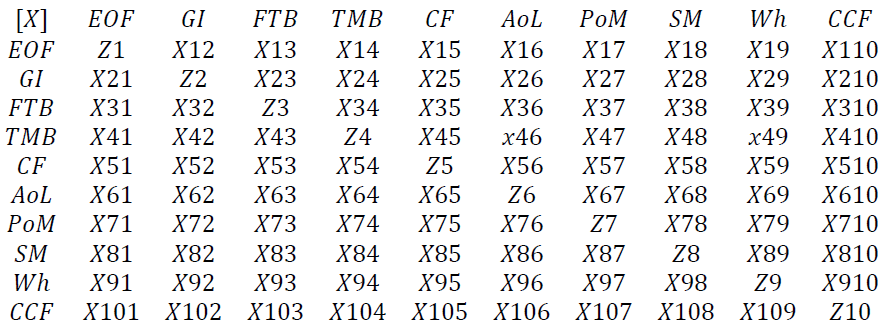
Any digraph consists of particular number of nodes N = {n_i}, where i is set of numbers {1 , 2 , 3 , ….. , M} and the set of directed Edges E = {x_ij}) Agrawal et al. (2016) . A node ni represents an ith attribute for the selection of satisfaction alternative, and edges represent the relative importance of these attributes. For example, if the attribute “i” is more important than the attribute “j” while comparing two attributes for their relative preference, then the vector or arrow or edge is directed from node “i” to node “j.” The value of preference is represented by x_ij. If the attribute “j” is more important than the attribute “i” then arrow or edge is directed from node “j” to node “i.” The value of preference is represented by x_ji. The function of the digraph is to create a visualization of the attributes and their relative preference to each other to help them analyze quickly. However, in case of the number of nodes or attributes increases then the visualization of such a graph may not deliver relevant results due to highly complex structures, thus in such cases where the number of nodes exceeds from the certain value after which the digraph may become complex the whole solution is converted into a matrix.

The matrix formed is a type of transformed digraph in the representation only. The matrix formed is Relative Importance Matrix Slack et al. (1994) where all off-diagonal elements discuss the relative preference of one attribute to the other. The diagonal elements give relative satisfaction or improvement alternative. Since the digraph or matrix is variable changing with the number of the attribute in observation, a standard matrix function is devised for the same. The function is called Permanent Function is computed rather than the determinant of the matrix. The mentioned function taken is because the determinant function of the matrix if computed may accompany the loss of information due to carrying negative signs. However, the complete information is considered in Permanent Function thus is wholly used as preferred Rao et al. (2007).

The study selected attributes are:

1. Ease of Filing (EoF).

2. Government Incentives (GI).

3. Foreign Trade Barriers (FTB).

4. Total Monetary Payment (TMP).

5. Customer Friendly (CF).

6. Availability of Loans (AoL).

7. Procurement of Materials (PoM),

8. Supplier Management (SM),

9. Warehousing (Wh),

10. Credit Cash Flow (CCF).

The digraph for the discussed ten attributes is shown in Figure 1 Agrawal et al. (2016).

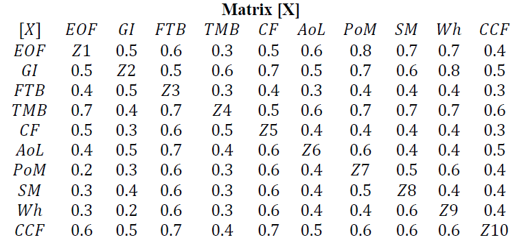
Since the representation of the digraph is complicated to decode from the visual interpretation of Figure 1, thus a matrix [X] has been developed for the more fundamental analysis of the same. The matrix produced is an M M type of matrix for ten different attributes consisting of the diagonal elements. The diagonal elements are represented by Z_ij, where i=j and in case of off-diagonal elements are represented by x_ij where i j.

The off-diagonal elements describe the relative satisfaction of each item and are the same for all alternatives or improvement alternatives. Diagonal elements indicate the need for improvement of an attribute for the given alternative and may differ for each choice.

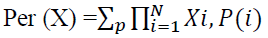
The permanent function of the above matrix is:

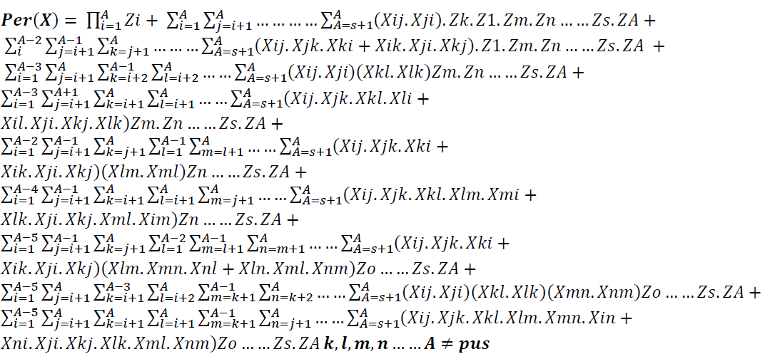
In general, the permanent of an M x M matrix, [A] with attributes x_ij defined by H Forbert et al. as:

Where the sum is the overall permutations P. Keeping in mind the end goal to ascertain the improvement points, a PC program for the M x M framework was composed in C++ computer language. The program takes a couple of minutes to run the query and figure the estimation of the permanent function value. The legitimate stream graph for creating and structure of the program is connected in the appendix (A1). The evaluation of the permanent function is referred to as the "Satisfaction Index" for the proposed consider. A well-ordered way to deal with applying GTMA identifies as takes after the following procedure.

Step1: Selection of cases to be reviewed and factors against which their performance is considered, as mentioned above in discussions of Relative importance matrix.

Step2: Define the relative performance of each case concerning each other. The value of off-diagonal elements is referred from this selection for filling (Table 2).

Table 2 The Scale of Relative Satisfaction for the Values
Portraiture	xij (Case A)	1-xij (Case B)
Equally satisfied in both cases	0.5	0.5
One factor(i) is slightly more satisfactory than other(j)	0.6	0.4
One factor(i) is strongly satisfactory than other(j)	0.7	0.3
One factor(i) is very strongly satisfactory than other(j)	0.8	0.2
One factor(i) is extremely high in satisfaction while other is least satisfied(j)	0.9	0.1
One factor(i) is exceptionally high in satisfaction while other is least satisfied(j)	1.0	0.0

Step3: Find out the importance of each factor in observation for individual cases on the parameterized scale Gerhart (2005). This step derives the value of diagonal elements in the matrix (Table 3).

Table 3 The Scale of Relative Satisfaction for the Values
Qualitative Significance	Scaled Value (Zi)
Exceptionally Bad	0.0
Extremely Bad	0.1
Very Bad	0.2
Bad	0.3
Below Average	0.4
Average	0.5
Above Average	0.6
Good	0.7
Very Good	0.8
Extremely Good	0.9
Exceptionally Good	1.0

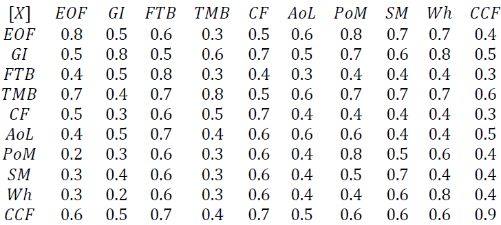
Step4: The step requires developing the required matrix for individual cases. The MxM matrix developed is Matrix [X]. The values in the matrix are the result of the parametrized scale chosen in step2 and step3 for filling in the value of non-diagonal and diagonal elements.

Step5: Calculating the permanent function best applicable to individual cases in observation.

Step6: This step requires the use of calculated permanent function value for the individual cases, as illustrated in the above equation Per(X). The same can be achieved by using manual calculation; however, for higher accuracy and time constraint, a C⁺⁺ program is used for the same. The compiler used is TurboC⁺⁺; however, another compiler like CodeBlocks can be used as well. This approach allows for a more straightforward comparison of each value to the different case values to determine the best performance in the cases.

Case Illustration

The sample case is based on the public survey, which was used to record various people as participants. The survey conducted through various online media sources ranging from non-finance services related to finance specialists. The survey was conducted to inspect the view of a variety of audiences ranging from industries specialist and ordinary people. The approach includes as many people as possible for acquiring distinct views and possible effects regarding observations with the changing backgrounds of the people, whether regarding their economic background, educational background, or professional background to better perceive the case in observation over the generalized market and economy.

The mode of information collection was chosen to be surveyed to facilitate the maximum amount of information collected over a smaller period with people of sparse backgrounds. The study conducted was in the form of a questionnaire with the no-costs to access links of Google Forms Link. The survey consisted of a total of 10 fundamental questions with 11 choices as a whole. The choices range from the Extremely Bad response to Extremely Good on the scale of 00 to 10 respectively and in-between. Each subject was further sub-branch for several cases to allow the participants to rank different parameters and their relative satisfaction in the presented cases. The cases mentioned are same as cases cited as alternatives in the methodology while each question parameter is same as the factor on which their relative performances are observed.

While the data collected in itself is allowably sorted to draw out the useful information correctly, the collected data is required to be further corrected to be able to provide more accurate information. The process can be solved via various methods to achieve higher accuracy, such as using median data values out of all participants; however, this type of approach may dilute the effectiveness in some cases. Similar results can be observed for other statistical data normalizations; thus it is profoundly prescribed to use an ample sample of the data to reduce the chances of high bias opinions and have a higher generalized point of view of the conventional markets. However, it is of advice that the sample space must always include people with mostly financial and managerial backgrounds or people having a basic understanding of economics and finances as a whole. This is to reduce the biased opinions out of the sample which may be shaped due to misinformation or other sources.

Here is an example is taken as the reference from many of participants in the survey to illustrate the basic idea of applying the discussed analytical method to find the best case out-performing relative to others on the selected specific factors. The expected result is suggested to be a significant value margin with maximum performance in the case of GST with the example of demonetization to be last with GST along with demonetization in the middle to near GST case values. The factors in observation can be reshuffled again and repeatedly for finding the best-suited elements to generate best and worst-performing factors combinations and sort-out the factors requiring maximum attention to examine for areas for possible implementations in future amendments.

STEP 1

This step entails the selection of the factors on which the various cases are being examined. The factors selected here are on the personal selection of the observer and can be varied upon the choice of another observer on the cases of the objective of the observer. The factors selected here are Ease of Filing (EoF), Government Incentives(GI), Foreign Trade Barriers(FTB), Total Monetary Payment(TMP), Customer Friendly(CF), Availability of Loans(AoL), Procurement of Materials(PoM), Supplier Management(SM), Warehousing(Wh) and Credit Cash Flow(CCF). A general summary of each alternative is provided in the summary table below for the review.

Also, along with the factors, the cases in observation selected are to be listed. The cases in selections here are:

Case I	Post-GST Period
Case II	Post-Demonetization Period
Case III	Post-Demonetisation period with successively implemented GST (Hypothetical)

STEP 2

Now the matrix X is filled with values of relative satisfaction based on the relative satisfaction index table. The values are selected for the off-diagonal elements by observer and survey results about the overall weight of each factor over the other. The values of diagonal elements are discussed ahead.

STEP 3

The values for the diagonal elements selected from the set scale mentioned are in the methodology. The values selected by the survey and participants' choices for the particular cases in each (Table 4 and Figure 2).

Table 4 Values of Diagonal Elements in the Individual Cases
Factors	Case I	Case II	Case III
EoF	0.8	0.3	0.8
GI	0.8	0.1	0.6
FTB	0.8	0.5	0.6
TMP	0.8	0.3	0.5
CF	0.7	0.2	0.5
AoL	0.6	0.1	0.1
PoM	0.8	0.1	0.5
SM	0.7	0.4	0.5
Wh	0.8	0.3	0.6
CCF	0.9	0.4	0.7

STEP 4

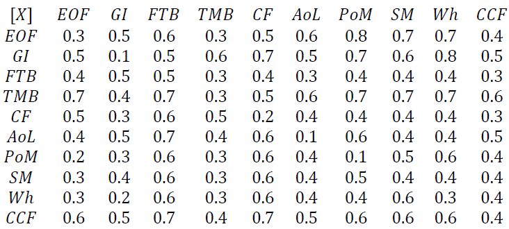
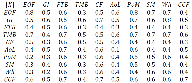
This step requires the fulfillment of the matrix values as required for the individual cases in the diagonal of the matrix developed in STEP 2. The values for Case I, Case II, and Case III is taken from the table developed in STEP 3.

Case I Matrix

Case II Matrix

Case III Matrix

STEP 5

The permanent function can be computed for each matrix, as described in the methodology. The value of the permanent function can be calculated using the Computer software programs as employed here. The value is computed using a C++ program in this research.

STEP 6

The Value of each case is calculated using the desired techniques and tools. The values here are arranged in the order of the cases computed.

CASE	Permanent Function Computed Value
Case I	4572.81
Case II	1626.06
Case III	3156.91

The values of the permanent function suggest a simple trend. The value of the permanent function in Case I is indicative of a high level of general satisfaction for the given selected factors in observation. These values correlate with the initial hypothesis that the new GST tax regime out to have a higher satisfaction index in overall comparison. The value of Case II is significantly lower as compared to the other cases, which also adds up to the initial hypothesis. The execution of the demonetization also received backlash for the way of executions and other types of after-effects that lingered in the commercial businesses for a more extended period. Case III was an altered hypothetical case in which the consideration was taken for if the demonetization had been implemented after the assimilation of GST in previous tax-regime structure. This case shows a significantly closer value to Case I, where only GST is implemented in typical routine markets. This value is significantly better than the case of application of demonetization in the previous ta regimes and thus clearly suggests the merits of GST and its robustness to allow for cushioning such unexpected blows to the current Indian economy (Figure 3).

Conclusion

The study undertaken in this paper uses the technique of GTMA (Graph Theory and Matrix Approach) for conducting a study about GST and its characteristics by individual factors which are variable by the type of study propose and the nature of observation required. The factors selected here Ease of Filing (EoF), Government Incentives (GI), Foreign Trade Barriers (FTB), Total Monetary Payment (TMP), Customer Friendly (CF), Availability of Loans (AoL), Procurement of Materials (PoM), Supplier Management (S), Warehousing (Wh) and Credit Cash Flow(CCF) are selected on the discretion of the observer as the motive of study was to find out about the collective satisfaction of people before and after GST implementation in India. The main reason for the selection of the GTMA technique is because of the ease of application, and the results generated are satisfactorily accurate. The highlight of the approach is the permanent function, employed to find an overall comparative value of each case.

Here the value generated by the permanent function is taken as “Overall Satisfaction Index.” The cases can be reiterated with different sets of factors in play and with different cases in question. All values generated and thus can be compared to find the places of improvements within the set of factors. This type of study is substantially free from constraints of the factors and cases in observation and allows for selecting the best cases along with better factors for application of the particular ideas in any the situation with the best possible outcome. The case discussed here is a culmination of data collected via means of an online survey. The results generated here are in support of the hypothesis of an observer than GST is better for upcoming Indian economy. The observations here can also help for amendments of the current GST status in the economy for broader and better fetching results. The technique used here is applicable for different types of applications as well and is not supposed to be specific to these types of analysis. Also, the results generated here can only be taken as a model representation of these types of analysis required a more substantial sample survey that may be employed here.

Acknowledgements

We much acknowledge the contributions of the subject editor, language expert, and reviewers for helping us in improving the quality of this article.

Funding

This research did not receive any specific grant from funding agencies in the public, commercial, or not-for-profit sectors.

References

1. Agrawal, S., Singh, R. K., & Murtaza, Q. (2016). Disposition decisions in reverse logistics: Graph theory and matrix approach. Journal of Cleaner Production, 137, 93-104.
2. Dani, S. (2016).  A Research Paper on an Impact of Goods and Service Tax (GST) on Indian Economy. Bus Eco J, 7, 264.
3. Deloitte GST Report retrieved from https://www2.deloitte.com/content/dam/Deloitte/in/Documents/tax/in-tax-gst-in-india- taking-stock-noexp.pdf.
4. Forbert, H., & Marx, D. (2003). Calculation of the permanent of a sparse positive matrix. Computer Physics Communications, 150(3), 267-273.
5. Gerhart, B. (2005). The (affective) dispositional approach to job satisfaction: Sorting out the policy implications. Journal of Organizational Behavior, 26(1), 79-97.
6. Goods and Service Tax. Retrieved from https://www.gst.gov.in/about/gst/history.
7. GST has not affected prices, but increased compliance burden: KPMG survey Retrieved from http://www.business- standard.com/article/economy-policy/gst-has-not-affected-prices-but-increased-compliance-kpmg-survey- 118022300762_1.html.
8. Jain, V., & Raj, T. (2016). Modeling and analysis  of  FMS  performance  variables  by  ISM,  SEM  and  GTMA  approach. International Journal of Production Economics, 171, 84-96.
9. Malik, S., Kumari, A., & Agrawal, S. (2015). Selection of locations of collection centers for reverse logistics  using GTMA. Materials Today: Proceedings, 2(4-5), 2538-2547.
10. Moorman, R.H., Niehoff, B.P., & Organ, D.W. (1993). Treating employees fairly and organizational citizenship behavior: Sorting the effects of job satisfaction, organizational commitment, and procedural justice. Employee responsibilities and rights journal, 6(3), 209-225.
11. Muduli, K., Govindan, K., Barve, A., Kannan, D., & Geng, Y. (2013). Role of behavioral factors in green supply chain management implementation in Indian mining industries. Resources, Conservation and Recycling, 76, 50-60.
12. Rao, R.V. (2007). Decision making in the manufacturing environment: using graph theory and fuzzy multiple attribute decision making methods. Springer Science & Business Media.
13. Rao, R.V., & Padmanabhan, K. K. (2007). Rapid prototyping process selection  using  graph  theory  and  matrix  approach. Journal of Materials Processing Technology, 194(1-3), 81-88.
14. Richard, P.J., Devinney, T. M., Yip, G. S., & Johnson, G. (2009). Measuring organizational performance: Towards methodological best practice. Journal of management, 35(3), 718-804.
15. Slack, N. (1994). The importance-performance matrix as a determinant of improvement priority. International Journal of Operations & Production Management, 14(5), 59-75.
16. Toloo, M., & Nalchigar, S. (2011). A new DEA method for supplier selection in presence of both cardinal and ordinal data. Expert Systems with Applications, 38(12), 14726-14731.
17. Venkatesh, A., Vulugundam, A. (2015). Impact on Of Gst on Supply Chain Strategy and Its Effect on Warehousing And Transportation http://www.mahindralogistics.com/logiquest/assets/pdf/LogiQuest_EastCoastExpress_NMIMS.PDF
18. Wagner, S.M., & Neshat, N. (2010). Assessing  the vulnerability of supply chains using graph theory. International Journal of Production Economics, 126(1), 121-129.
19. Yang, J.L., & Tzeng, G.H. (2011).  An integrated MCDM technique combined with DEMATEL for a novel cluster-weighted with ANP method. Expert Systems with Applications, 38(3),1417-1424.