Keywords

Performance Appraisal, Sustainable Supply Chain, ANP, TOPSIS

Introduction

Supply chain management (SCM) is known as one of the underlying foundations for the implementation of electronic business in the world. Supply Chain Management is a phenomenon that emerged in the 1990s and does its task in such a way that customers can receive reliable and fast services with high-quality products at minimum cost (Makui, 2000).

Supply chain consists of all the steps directly or indirectly involved in fulfillment of customers' needs and includes a range of primary suppliers to end customers. Three main information are, physical and financial flows exist in this chain. This flow of information and knowledge also gives orientation to the two financial and physical elements. Therefore, it is very important to evaluate knowledge management and identify how to apply it in the organization (Yu et al., 2013).

In the turbulent and changing world of today, the only thing that doesn’t change is the change. To survive in today's competitive world, organizations must prepare themselves to compete (Porter & Michael, 2001). On the other hand, in today’s economy, competition is no longer in the form of the firm s competition against another firm, but it’s the supply chains which compete with each other. The supply chain management is responsible for material flows in the community and serves as an exchange of materials and energy with the environment. The impacts of SCM should be specified related to the three main aspects of sustainability: environmental performance, social responsibility and economic contribution. Today, it is mainly focused on the economic aspect, through evaluating some of the best or well-known methods. With the increasing use of the Internet as one of the main tools of business and the sharp rise in competition, more sophisticated supply chains have emerged which include several layers (the supplier layer, customer layer etc.) and produce different products (Nikpour & Salajegh, 2010). The Oil, Gas, and Petrochemical Investment Corporation (TAPICO) are one of the affiliated companies of the Social Security Investment Company (SHASTA) which has developed over a 13-year period. With a total of 32 management and affiliated companies in the oil, gas, petrochemical, rubber and cellulose industries, TAPICO has a significant contribution in the mentioned economic sector. Among the approaches used in each of these sectors and sub-companies, is the sustainability approach in the supply chain. This study will help TOPICO Group companies identify the focused solutions and key assessment indicators for better management of the sustainable supply chain. The core indicators of supply chain assessment will be identified. Also, at the end of this applied study, according to the output of the network analysis process, the assessment of the existing suppliers will be carried on. So this study will answer the following basic questions: What are the most important indicators of performance assessment of sustainable supply chain management in TAPICO? How the pattern of relationships among these elements and what is the importance of each? What are the top priorities of TAPICO's suppliers based on existing indicators and their importance?

Literature Review

Teimoori (2000) conducted a study entitled

“Providing models for supply chain management systems with cognitive and analytical studies”,

In which he investigated and determined the critical factors of success as well as the key criteria of platform-based supply chain performance. He came to the conclusion that the components structure and capabilities of the supply network, globalization, the product architecture and engineering, business management and industry structure have a direct impact with the platform-based supply chains and there is a significant relationship between them. The results of this study may be consistent with those of the present research in some respect.

Olfat & Barati (2012) dealt in a study with the requirements of green supply chain management fulfillment in the automotive industry of Iran, aiming to identify the requirements (stimulators, obstacles, actions and results) for achieving a green supply chain management. They came to 5 conclusions including positive economic results, negative economic results, environmental results, production performance improvement and stakeholders' satisfaction, and used the MADM method to prioritize and determine the importance degree and used TOPSIS method in multi-criteria decision-makings. Sharma & Bhagwat (2007) conducted a study entitled

“An integrated BSC-AHP approach for supply chain management evaluation”.

The results of their research suggest that measuring performance at the strategic level is more important than the tactical and operational levels, and customer is the most important prospect in the supply chain performance appraisal.

In a study, Sahebi et al. (2014) has investigated the use of OFD and TOPSIS fuzzy modulation approaches in selecting the supplier. In this study, by combining fuzzy logic and quality house, qualitative criteria were considered in the process of selecting suppliers in Saipa Sazeh Gostar Company. The TOPSIS method was then adopted to consider quantitative measures. Eventually, with the combination of FUZZY-QFD and TOPSIS techniques, Nissan's suppliers were selected and ranked in the company. Considering both qualitative and quantitative criteria is an important point in this research and the methodology used is also an innovative aspect. In line with the research objectives, the most important qualitative and quantitative criteria for selecting the suppliers in this company were determined according to the literature of the subject and consulting with the team of experts in the company. Performance history, management competencies, management stability, quality, geographic location, supplier flexibility, delivery function, environmental management, ability to send parts, after sales service, technical and technological capability, ease of communication, supply diversity, average returns of goods and production costs (Sahebi, 2014).

In a study, Amiri et al. (2009) have analyzed the factors affecting supply chain performance with the combined approaches of Fuzzy confirmatory factorization and fuzzy TOPSIS (Case study: Shiraz Food Industry companies of industrial park. The method used in this study is a combination of two approaches of confirmatory factor analysis and fuzzy TOPSIS. In line with the aim of the present study, the factors affecting supply chain performance were identified and studied. After reviewing the research literature, 26 factors affecting supply chain performance were identified. In the first stage, regarding the opinions of academic and industry experts through confirmatory factor analysis, 22 important factors were identified and in the second stage, Shannon's entropy technique was used to gain the weight of the importance of expert opinions and Fuzzy TOPSIS technique was used to rank the factors affecting supply chain performance. The results of this study show that the factors of “supplier selection”, “timely delivery”, “purchase order cycle time”, “quality” and “power” are the most important factors affecting supply chain performance in this industry and ranked higher than other factors. In a study titled the combined approach of BSC and AHP to assess the performance of the supply chain management.

Sharma & Bhagwat (2007) presented a combination approach of BSC and AHP to assess the performance of the supply chain management. The results of the research indicate that the measurement of performance at the strategic level is more important than the other two levels, namely, tactical and operational levels, and the customer is the most important perspective in assessing the supply chain performance. According to the results of the research, the executive action is consistent with the present research from the point of view of the sub-criteria sub-criterion

Park et al. (2010) stated the supplier's assessment criteria based on the shopping strategy of Quartz Company. There are three assessment groups in this company: quality, cost and delivery for performance assessment; technology and management to assess capabilities; and collaboration to assess cooperative relationships.

Amin et al. (2011) categorized the criteria into internal and external categories, each of which categorized as quantitative (QN) and qualitative (QL) criteria, as follows:

1. The internal criteria are: unit cost (QN), quality (QL), timely delivery rate (QN), management stability (QL).

2. External criteria include: mutual trust (QL), geographical location strength (QL), International Relations (QL).

Rostamzadeh et al. (2018) aim the establishment a framework for assessing supply chain risk management (SSCRM). For this purpose, an integrated fuzzy multi-criteria decision making (MCDM) approach based on prioritized techniques with the ideal solution (TOPSIS) and criterion importance through correlation methods between two criteria (CRITIC) is proposed. Literature was examined and potential criteria were identified. Criteria were filtered through a special panel. The seven main criteria and the forty four sub-criteria were presented for the SSCRM framework. Most of the following criteria are found in each group: the risks of machinery and equipment, major supplier failures, demand fluctuations, government policy risks, IT security, economic issues, and inadequate sewage intrusion. Among these criteria, the economic criterion is consistent with the current research.

Methodology

Supply Chain

Since the main purpose of this research is to identify and rank the criteria of appraisal of sustainable supply chain management performance with a multi-criteria decision-making approach, it can be said that the present research is an applied research in terms of objective. On the other hand, since library study and fieldwork methods such as questionnaire have been used in this research, it can be said that this is a descriptive-survey research in terms of nature and method.

This research has used interviews and questionnaire tools to collect the research data. Questionnaire No. 1 is an expert questionnaire to prioritize criteria and sub-criteria based on the paired comparison. These questionnaires are based on a 9-hour span. In this research, a paired hourly model is used to design an expert questionnaire. Using this model, the relative significance of the criteria is estimated using a pairwise comparison. For scoring, the fuzzy equivalent of the nine-hour scale is used, which is shown in Table 1.

Table 1: Fuzzy Spectrum Equivalent to the Nine-Hour Scale
The verbal expression compares i to j	Fuzzy equivalent	Reverse fuzzy equivalent
Equally preferred	(1, 1, 1 )	(1, 1, 1)
Midway	(1, 2, 3 )	(1/3, 1/2, 1)
(Moderetely preferred (Slightly Better	(2, 3, 4 )	(1/4, 1/3, 1/2)
Midway	(3, 4, 5 )	(1/5, 1/4, 1/3)
Strongly preferred	(4, 5, 6 )	(1/6, 1/5, 1/4)
Midway	(5, 6, 7 )	(1/7, 1/6, 1/5)
Very strongly Preferred	(6, 7, 8 )	(1/8, 1/7, 1/6)
Midway	(7, 8, 9 )	(1/9, 1/8, 1/7)
Extremely preferred	(9, 9, 9 )	(1/9, 1/9, 1/9)

In the present study, because of multi criteria decision making and research in operation, the community is considered to be experts and senior experts in the study area. In this study, the network analysis process technique was used to prioritize the criteria. Habibi (2014) believes that ten experts are sufficiently suited for comparative studies.

Therefore, the circle of expert’s selection is very limited and as a result, ten eligible individuals are selected as examples of the study.

Data Analysis

This study has been conducted in several stages and using several techniques. In this study, the analytic network process (ANP) has been used to determine and prioritize the indicators. For this purpose, the pair-wise comparison matrix has been used to determine the weights of the criteria. Finally, TOPSIS technique has been used to prioritize the research options. The calculations related to the ANP technique have also been made using the Super Decision software.

Prioritization of the Criteria and Sub-Criteria of the Model Using ANP Technique

The main criteria of the study include: economic factors, environmental factors, and infrastructural and cultural factors. Several sub-criteria were identified for each one of the main criteria, and 21 sub-criteria were identified on the whole presented in Table 2.

Table 2 The Criteria and Sub-Criteria of the Research
Main criteria		Sub-criteria	Symbol
Economic factors	C1	Automation	S11
		The cost of supply chain	S12
		The return cost	S13
		Product durability	S14
		Cost of design	S15
		Cost of resources	S16
		Production cost	S17
		Flexibility of supply	S18
Environmental factors	C2	Integration and participation	S21
		Integration of the processes	S22
		Understanding the market disequilibrium	S23
		Dangerous factors of the workplace and community	S24
		Environmental pollution	S25
Social factors	C3	Performance of the business and marketing sector	S31
		Timely and suitable delivery	S32
		Quality improvement	S33
		Rapid delivery	S34
		Customers' status	S35
		Mutual trust and communication	S36
		Humanitarian laws	S37
		Culture and technology development	S38

The criteria and sub-criteria model with ANP technique is shown in Figure 1. Moreover, the criteria and sub-criteria of the research have been named with numeric index as Error! Reference source not found, so that they can be easily tracked and studied during the research flow.

We have used the ANP technique in this study in order to determine the weights of the criteria and indicators of the model. The analysis was made with the following steps:

i. Prioritization of the main criteria based on the objective via pair-wise comparison,

ii. Prioritization of each one of the sub-criteria in its respective cluster through pa pair-wise comparison,

iii. Calculation of the initial super matrix, the weighted super matrix and the limit super matrix.

Prioritization of the Main Criteria Based on the Objective

For the network analysis, we first made a pair-wise comparison of the main criteria based on the objective (sustainable supply chain performance improvement). Pair-wise comparison is very simple and all elements of each cluster should be mutually compared. Thus, if there is n elements in a cluster, comparisons will be made. As there are three criteria here, the number of the comparisons will be:

Therefore, three pair-wise comparisons were made from the perspective of a group of experts. The experts' views were quantified using the fuzzy scale. Then, their views were fuzzed. We used the geometric mean method in ANP approach in order to Tajmia the experts' views. Based on the results of the Tajmia of experts' views, the pair-wise comparison matrix can be presented as follows in the Table 3.

Table 3 The Pair-Wise Comparison Matrix of the Main Criteria of the Research
	Social factors	Environmental factors	Social Economic factors
Economic factors	(1, 1, 1)	(1.14, 1.41, 1.72)	(1.28, 1.75, 2.32)
Environmental factors	(0.58, 0.71, 0.88)	(1, 1, 1)	(1.02, 1.37, 1.68)
Social factors	(0.43, 0.57, 0.78)	(0.59, 0.73, 0.98)	(1, 1, 1)

The fuzzy extension of each criterion will be as follows:

1. Fuzzy extension of column 1: (1, 1, 1) ⊕ (1.14, 1.41, 1.72) ⊕ (1.28, 1.75, 2.32)=(3.42, 4.16, 5.04)

2. Fuzzy extension of column 2: (0.58, 0.71, 0.88) ⊕ (1, 1, 1) ⊕ (1.02, 1.37, 1.68)=(2.6, 3.09, 3.56)

3. Fuzzy extension of column 3: (0.43, 0.57, 0.78) ⊕ (0.59, 0.73, 0.98) ⊕ (1, 1, 1)=(2.03, 2.3, 2.76)

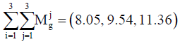
Then, the fuzzy sum of the total elements of the column is calculated as follows:

The total elements of the column of preferences of the main criteria are as follows:

To normalize the preferences of each criterion, we should divide the total sum of the values of each criterion into the total sum of all preferences (elements of the column). Therefore, the fuzzy sum of each column is multiplied by the reverse sum. The reverse sum should be calculated.

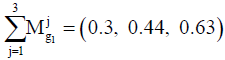
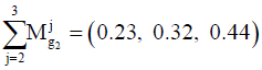
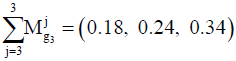
Therefore, the results of normalizing the values will be as follows: C1=(0.3, 0.44, 0.63); C2=(0.23, 0.32, 0.44); C3=(0.18, 0.24, 0.34).

The values obtained are the fuzzy and normalized weights of the main criteria. In the final step, the values were defuzzified and the Crisp Number was calculated. The calculations made for determining the priorities of the main criteria are presented in Table 4.

Table 4 Defuzzification of the Normal Weights of the Main Variables
Crisp	X1max	X2max	X3max	Defuzzy	Normal
Economic factors	0.454	0.45	0.445	0.454	0.437
Environmental factors	0.331	0.329	0.327	0.331	0.319
social factors	0.254	0.251	0.248	0.254	0.244

Based on the eigenvector obtained:

1. Economic factors have the highest priority with the normal weight of 0.437.

2. Environmental factors have the second priority with the normal weight of 0.319.

3. Social factors have the lowest priority with the normal weight of 0.244.

The inconsistency rate of the comparisons was obtained as 0.001, and therefore we can rely on the comparisons as it is smaller than 0.1.

Comparison and prioritization of the sub-criteria

In the second step of ANP technique, the sub-criteria relating to each criterion were compared in pairs.

Prioritization of the economic sub-criteria

First we present the calculations made to determine the priority of the economic sub-criteria. The economic sub-criteria include: automation, supply chain costs, cost of return, product durability, cost of design, cost of resources, production cost and flexibility of supply.

Since this criterion consists of 8 indicators, 28 pair-wise comparisons were made. The inconsistency rate of the comparisons was obtained as 0.083, and therefore we can rely on the results as it is smaller than 0.1. The experts' views were first collected in the pc pair-wise comparison of each one of the economic criteria. Then, the obtained values were tajmied via calculation of the fuzzy mean. The pair-wise comparison matrix of the social factors' components are presented in Table 5

Table 5 Pairwise Comparison Matris of Economic Sub-Criteria
	S11	S12	S13	S14	S15	S16	S17	S18
SSS	(1, 1, 1)	(1.4, 1.82, 2.26)	(2.46, 3.09, 3.76)	(2.75, 3.38, 3.98)	(2.83, 3.87, 4.9)	(0.57, 0.67, 0.81)	(2.64, 3.68, 4.7)	(1.71, 1.89, 2.08)
S12	(0.44, 0.55, 0.72)	(1, 1, 1)	(1.71, 1.89, 2.08)	(2.46, 3.5, 4.52)	(1.87, 2.31, 2.81)	(0.49, 0.61, 0.79)	(2.35, 2.69, 3.07)	(2.46, 3.5, 4.52)
S13	(0.27, 0.32, 0.41)	(0.48, 0.53, 0.58)	(1, 1, 1)	(2.81, 3.27, 3.78)	(2.23, 2.88, 3.57)	(0.7, 0.92, 1.2)	(0.93, 1.21, 1.6)	(2, 3, 4)
S14	(0.25, 0.3, 0.36)	(0.22, 0.29, 0.41)	(0.26, 0.31, 0.36)	(1, 1, 1)	(0.21, 0.25, 0.31)	(0.39, 0.48, 0.59)	(2.56, 3.62, 4.65)	(0.21, 0.27, 0.38)
S15	(0.2, 0.26, 0.35)	(0.36, 0.43, 0.54)	(0.28, 0.35, 0.45)	(3.25, 4.04, 4.81)	(1, 1, 1)	(0.17, 0.2, 0.25)	(0.6, 0.73, 0.87)	(0.35, 0.42, 0.54)
S16	(1.23, 1.5, 1.74)	(1.27, 1.63, 2.02)	(0.84, 1.09, 1.43)	(1.71, 2.1, 2.55)	(4, 5, 5.99)	(1, 1, 1)	(2.46, 3.5, 4.52)	(3.67, 4.75, 5.79)
S17	(0.21, 0.27, 0.38)	(0.33, 0.37, 0.43)	(0.63, 0.83, 1.07)	(0.22, 0.28, 0.39)	(1.15, 1.37, 1.66)	(0.22, 0.29, 0.41)	(1, 1, 1)	(1.52, 2.1, 2.75)
S18	(0.48, 0.53, 0.58)	(0.22, 0.29, 0.41)	(0.25, 0.33, 0.5)	(2.64, 3.68, 4.7)	(1.87, 2.37, 2.89)	(0.27, 0.21, 0.27)	(0.36, 0.48, 0.66)	(1, 1, 1)

After the formation of the matrix of pairwise comparison, the fuzzy sum of each row is calculated. Therefore, the fuzzy expansion of the preferences of each of the sub-criteria is as follows

1. Fuzzy expansion of row 1 (1, 1, 1)⊕(1.4, 1.82, 2.26)⊕(2.46, 3.09, 3.76)⊕(2.75, 3.38, 3.98)⊕(2.83, 3.87, 4.9)⊕(0.57, 0.67, 0.81)⊕(2.64, 3.68, 4.7)⊕(1.71, 1.89, 2.08)=(15.36, 19.4, 23.49)

2. Fuzzy expansion of row 2 (0.44, 0.55, 0.72)⊕(1, 1, 1)⊕(1.71, 1.89, 2.08)⊕(2.46, 3.5, 4.52)⊕(1.87, 2.31, 2.81)⊕(0.49, 0.61, 0.79)⊕(2.35, 2.69, 3.07)⊕(2.46, 3.5, 4.52)=(12.79, 16.05, 19.5)

3. Fuzzy expansion of row 3 (0.27, 0.32, 0.41)⊕(0.48, 0.53, 0.58)⊕(1, 1, 1)⊕(2.81, 3.27, 3.78)⊕(2.23, 2.88, 3.57)⊕(0.7, 0.92, 1.2)⊕(0.93, 1.21, 1.6)⊕(2, 3, 4)=(10.42, 13.13, 16.13)

4. Fuzzy expansion of row 4 (0.25, 0.3, 0.36)⊕(0.22, 0.29, 0.41)⊕(0.26, 0.31, 0.36)⊕(1, 1, 1)⊕(0.21, 0.25, 0.31)⊕(0.39, 0.48, 0.59)⊕(2.56, 3.62, 4.65)⊕(0.21, 0.27, 0.38)=(5.12, 6.5, 8.05)

5. Fuzzy expansion of row 5 (0.2, 0.26, 0.35)⊕(0.36, 0.43, 0.54)⊕(0.28, 0.35, 0.45)⊕(3.25, 4.04, 4.81)⊕(1, 1, 1)⊕(0.17, 0.2, 0.25)⊕(0.6, 0.73, 0.87)⊕(0.35, 0.42, 0.54)=(6.2, 7.43, 8.8)

6. Fuzzy expansion of row 6 (1.23, 1.5, 1.74)⊕(1.27, 1.63, 2.02)⊕(0.84, 1.09, 1.43)⊕(1.71, 2.1, 2.55)⊕(4, 5, 5.99)⊕(1, 1, 1)⊕(2.46, 3.5, 4.52)⊕(3.67, 4.75, 5.79)=(16.17, 20.56, 25.04)

7. Fuzzy expansion of row 7 (0.21, 0.27, 0.38)⊕(0.33, 0.37, 0.43)⊕(0.63, 0.83, 1.07)⊕(0.22, 0.28, 0.39)⊕(1.15, 1.37, 1.66)⊕(0.22, 0.29, 0.41)⊕(1, 1, 1)⊕(1.52, 2.1, 2.75)=(5.27, 6.51, 8.08)

8. Fuzzy expansion of row 8 (0.48, 0.53, 0.58)⊕(0.22, 0.29, 0.41)⊕(0.25, 0.33, 0.5)⊕(2.64, 3.68, 4.7)⊕(1.87, 2.37, 2.89)⊕(0.27, 0.21, 0.27)⊕(0.36, 0.48, 0.66)⊕(1, 1, 1)=(7.09, 8.88, 11.02)

In short, it will be represented as in Table 6.

Table 6 Reversal of Total Preferences
Economic sub-criteria	Fuzzy expansion	Normal
S11	(15.36, 19.4, 23.49)	(0.12, 0.19, 0.31)
S12	(12.79, 16.05, 19.5)	(0.1, 0.16, 0.25)
S13	(10.42, 13.13, 16.13)	(0.08, 0.13, 0.21)
S14	(5.12, 6.5, 8.05)	(0.04, 0.07, 0.11)
S15	(6.2, 7.43, 8.8)	(0.05, 0.07, 0.11)
S16	(16.17, 20.56, 25.04)	(0.13, 0.21, 0.33)
S17	(5.27, 6.51, 8.08)	(0.04, 0.07, 0.11)
S18	(7.09, 8.88, 11.02)	(0.06, 0.09, 0.14)
Total preference	(78.42, 98.46, 120.11)
Reverse Total Preferences	(0.008, 0.01, 0.013)

The results of the calculation of the defuzzified values of the weights of economic sub-criteria are presented in Table 7 & Figure 2.

Table 7 The Defuzzified Values of the Weights of Economic Sub-Criteria
Crisp	X1max	X2max	X3max	Defuzzy	Normal
Automation	0.207	0.204	0.201	0.207	0.196
Supply chain cost	0.172	0.17	0.167	0.172	0.163
Cost of return	0.141	0.139	0.136	0.141	0.134
Product durability	0.07	0.069	0.068	0.07	0.066
Cost of design	0.079	0.078	0.077	0.079	0.075
Cost of resources	0.22	0.217	0.213	0.22	0.208
Production cost	0.071	0.069	0.068	0.071	0.067
Flexibility of supply	0.096	0.095	0.093	0.096	0.091

• The cost of resources index has the highest priority with the normal weight of 0.208.

• The automation index has the second priority with the normal weight of 0.196.

• The Supply Chain cost index has the third priority with the normal weight of 0.163.

Determining the priority of the environmental variables

Environmental sub-criteria include: integration and participation, integration of the processes, understanding the market disequilibrium, dangerous factors for the workplace and community, and environmental pollution. Because this index consists of five indices, 10 pair-wise comparisons were thus made. The inconsistency rate of the comparisons was 0.072, and we can thus rely on the results because it was smaller than 0.1. The results of the pair-wise comparisons of the Indies of other environmental sub-criteria are presented in Table 8.

Table 8  The Pair-Wise Comparison Matrix of the Environmental Sub-Criteria
	S21	S22	S23	S24	S25
S21	(1, 1, 1)	(0.52, 0.65, 0.85)	(1.4, 1.79, 2.22)	(1.32, 1.68, 2.04)	(1.19, 1.45, 1.78)
S22	(1.18, 1.53, 1.92)	(1, 1, 1)	(1.64, 1.92, 2.2)	(2.42, 3.06, 3.7)	(0.84, 1.04, 1.33)
S23	(0.45, 0.56, 0.71)	(0.45, 0.52, 0.61)	(1, 1, 1)	(1.52, 1.94, 2.48)	(1.25, 1.49, 1.78)
S24	(0.49, 0.6, 0.76)	(0.27, 0.33, 0.41)	(0.4, 0.52, 0.66)	(1, 1, 1)	(1.71, 2.07, 2.51)
S25	(0.56, 0.69, 0.84)	(0.75, 0.96, 1.2)	(0.56, 0.67, 0.8)	(0.59, 0.48, 0.59)	(1, 1, 1)

Fuzzy expansion calculations

1. Fuzzy row expansion 1 (1, 1, 1)⊕(0.81, 1.01, 1.25)⊕(1.24, 1.4, 1.6)⊕(0.93, 1.2, 1.49)⊕(0.48, 0.55, 0.64)=(4.47, 5.17, 5.99)

2. Fuzzy row expansion 2 (0.8, 0.99, 1.23)⊕(1, 1, 1)⊕(1.6, 1.96, 2.34)⊕(1.34, 1.74, 2.19)⊕(0.82, 0.97, 1.17)=(5.55, 6.66, 7.92)

3. Fuzzy row expansion 3 (0.62, 0.71, 0.8)⊕(0.43, 0.51, 0.63)⊕(1, 1, 1)⊕(1.25, 1.53, 1.83)⊕(0.75, 0.89, 1.06)=(4.05, 4.65, 5.33)

4. Fuzzy row expansion4 (0.67, 0.83, 1.07)⊕(0.46, 0.57, 0.75)⊕(0.54, 0.65, 0.8)⊕(1, 1, 1)⊕(0.57, 0.7, 0.87)=(3.24, 3.76, 4.49)

5. Fuzzy row expansion 5 (1.57, 1.81, 2.08)⊕(0.86, 1.03, 1.22)⊕(0.94, 1.13, 1.33)⊕(1.76, 1.43, 1.76)⊕(1, 1, 1)=(6.13, 6.4, 7.39).

Due to the length of the fuzzy calculations and the same steps taken for setting the priorities of each of the sub-criteria in this study (Table 9), we have avoided repeating them in this section. The priority of the sub-criteria of each cluster is displayed in Figure 3.

Table 9 Calculation of the Final Weight of the Environment Sub-Criteria
	X1max	X2max	X3max	Defuzzy	Normal
Integration and participation	0.237	0.235	0.233	0.237	0.227
Integration of the processes	0.307	0.305	0.303	0.307	0.294
Understanding the market disequilibrium	0.199	0.198	0.196	0.199	0.191
Dangerous factors for the workplace and community	0.163	0.162	0.16	0.163	0.156
Environmental pollution	0.138	0.137	0.136	0.138	0.132

Due to the length of the fuzzy calculations and the same steps taken for setting the priorities of each of the sub-criteria in this study (Table 9), we have avoided repeating them in this section. The priority of the sub-criteria of each cluster is displayed in Figure 3.

• Integration of the processes has the first priority with the normal weight of 0.294.

• Integration and participation has the second priority with the normal weight of 0.227.

• Understanding the market disequilibrium has the third priority with the normal weight of 0.191.

Setting the priority of the infrastructural and cultural sub-criteria

Social sub-criteria include: mutual trust and communication, timely and suitable delivery, quality improvement, rapid delivery, customers' status, humanitarian laws, performance of the business and marketing sectors, and culture and technology development. Because this criterion has 8 indicators, 28 pair-wise comparisons were thus made. The inconsistency rate of the comparisons was 0.008, and we can thus rely on the results because it was smaller than 0.1. The results of the pair-wise comparisons of the Indies of other infrastructural and cultural sub-criteria are presented in Table 10 and a summary of the calculation of the final weight of the structural and cultural factors are presented in Table 11 & Figure 4.

Table 10 Pair-Wise Comparison Matrix of Infrastructural & Cultural Sub-Criteria
	S31	S32	S33	S34	S35
S31	(1, 1, 1)	(0.6, 0.76, 0.91)	(0.87, 1.09, 1.3)	(0.69, 0.95, 1.32)	(0.64, 0.79, 1.02)
S32	(1.1, 1.32, 1.66)	(1, 1, 1)	(0.72, 0.87, 1.07)	(1.3, 1.56, 1.86)	(0.93, 1.17, 1.44)
S33	(0.77, 0.92, 1.15)	(0.93, 1.14, 1.39)	(1, 1, 1)	(1.02, 1.35, 1.72)	(0.71, 0.91, 1.13)
S34	(0.76, 1.05, 1.46)	(0.54, 0.64, 0.77)	(0.58, 0.74, 0.98)	(1, 1, 1)	(0.7, 0.85, 1.03)
S35	(0.98, 1.27, 1.57)	(0.7, 0.85, 1.07)	(0.88, 1.1, 1.4)	(0.97, 1.17, 1.43)	(1, 1, 1)
S36	(1.18, 1.46, 1.89)	(1.12, 1.48, 1.88)	(1.17, 1.41, 1.8)	(1.35, 1.65, 1.95)	(1.33, 1.69, 2.02)

Table 11 Calculation of the Final Weight of the Structural & Cultural Factors
Crisp	X1max	X2max	X3max	Defuzzy	Normal
Mutual trust and communication	0.15	0.147	0.144	0.15	0.139
Timely and suitable delivery	0.146	0.143	0.14	0.146	0.135
Quality improvement	0.111	0.109	0.107	0.111	0.103
Rapid delivery	0.122	0.12	0.117	0.122	0.112
Customers' status	0.153	0.151	0.149	0.153	0.142
Humanitarian laws	0.161	0.158	0.155	0.161	0.149
Performance of the business and marketing sectors	0.138	0.135	0.131	0.138	0.127
Culture and technology development	0.101	0.099	0.097	0.101	0.094

Fuzzy expansion calculations

1. Fuzzy row expansion1 (1, 1, 1)⊕(0.91, 1.26, 1.81)⊕(0.96, 1.3, 1.74)⊕(0.91, 1.22, 1.66)⊕(0.91, 1.25, 1.69)⊕(0.73, 0.96, 1.2)⊕(0.52, 0.72, 1.06)⊕(1.08, 1.46, 1.88)=(7.03, 9.17, 12.05)

2. Fuzzy row expansion2 (0.55, 0.79, 1.1)⊕(1, 1, 1)⊕(1.08, 1.46, 1.88)⊕(0.97, 1.18, 1.44)⊕(0.72, 0.92, 1.2)⊕(0.83, 1.15, 1.59)⊕(0.88, 1.25, 1.82)⊕(0.92, 1.18, 1.51)=(6.96, 8.93, 11.54)

3. Fuzzy row expansion 3 (0.57, 0.77, 1.04)⊕(0.53, 0.69, 0.92)⊕(1, 1, 1)⊕(0.64, 0.84, 1.09)⊕(0.65, 0.86, 1.14)⊕(0.45, 0.65, 0.89)⊕(0.77, 1.04, 1.34)⊕(0.76, 0.99, 1.3)=(5.38, 6.83, 8.72)

4. Fuzzy row expansion 4 (0.6, 0.82, 1.1)⊕(0.7, 0.85, 1.03)⊕(0.92, 1.2, 1.56)⊕(1, 1, 1)⊕(0.63, 0.78, 1.04)⊕(0.63, 0.73, 0.84)⊕(0.65, 0.97, 1.4)⊕(1, 1.2, 1.45)=(6.12, 7.53, 9.41)

5. Fuzzy row expansion 5 (0.59, 0.8, 1.1)⊕(0.83, 1.08, 1.39)⊕(0.87, 1.17, 1.54)⊕(0.96, 1.28, 1.6)⊕(1, 1, 1)⊕(0.98, 1.26, 1.49)⊕(0.7, 0.93, 1.28)⊕(1.47, 2.05, 2.55)=(7.41, 9.57, 11.95)

6. Fuzzy row expansion 6 (0.84, 1.04, 1.37)⊕(0.63, 0.87, 1.21)⊕(1.13, 1.54, 2.21)⊕(1.2, 1.37, 1.58)⊕(0.67, 0.79, 1.02)⊕(1, 1, 1)⊕(1, 1.37, 1.8)⊕(1.35, 1.97, 2.49)=(7.81, 9.96, 12.69)

7. Fuzzy row expansion 7 (0.94, 1.38, 1.91)⊕(0.55, 0.8, 1.14)⊕(0.75, 0.96, 1.3)⊕(0.71, 1.03, 1.55)⊕(0.78, 1.07, 1.43)⊕(0.56, 0.73, 1)⊕(1, 1, 1)⊕(0.96, 1.35, 1.88)=(6.25, 8.32, 11.2)

8. Fuzzy row expansion 8 (0.53, 0.69, 0.92)⊕(0.66, 0.85, 1.08)⊕(0.77, 1.01, 1.32)⊕(0.69, 0.84, 1)⊕(0.39, 0.49, 0.68)⊕(0.74, 0.51, 0.74)⊕(0.53, 0.74, 1.04)⊕(1, 1, 1)=(5.32, 6.11, 7.78)

• Mutual trust and communication has the highest priority with the normal weight of 0.149.

• Customers' status has the second priority with the normal weight of 0.142.

• Performance of the business and marketing sectors has the third priority with the normal weight of 0.139.

The Final Priority of Indicators with FANP Technique

Calculations of un-weighted weighted and limit super matrixes

To determine the final weight, the output of the comparison of the main criteria based on the purpose and the internal relationships between the criteria are presented in a super-matrix. This super-matrix is called a primary or unbalanced super-matrix. In order to achieve the calculated priorities in the final W, the general requirements of a system with interactions, internal-priority vectors must be entered in the appropriate columns of a matrix. As a result, a super-matrix, each section of which shows the relationship between two clusters in a system, will be achieved. According to the relationships identified in this study, the primary matrix of this study will be as follows:

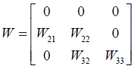
W22 shows the significance of each of the main criteria based on the purpose. In this matrix, W21 vector is the vector which shows the paired comparison of the relationships between its main criteria. W32 vector shows the significance of each of sub-criteria in the related cluster. The zero strings also indicate the ineffectiveness of the factors at the intersection of the rows and columns.

To determine the final weight, the output of comparison of the main criteria based on the objectives and the interrelations among the criteria are presented in a super matrix. This super matrix is called primary or un-weighted super matrix. The network pattern of the model has been designed using ANP technique in Super Decision Software. The un-weighted (primary) super matrix (Table 12 A&B) has been obtained based on the calculations from the first to the fourth steps.

Table 12A Primary (Unweighted) Super Matrix
3 Alternatives
S38	S37	S36	S35	S34	S363	S32	S31	S25	S24	S23	S22	S21
0.000	0.000	0.000	0.000	0.000	0.000	0.000	0.000	0.000	0.000	0.000	0.000	0.000
0.000	0.000	0.000	0.000	0.000	0.000	0.000	0.000	0.000	0.000	0.000	0.000	0.000
0.000	0.000	0.000	0.000	0.000	0.000	0.000	0.000	0.000	0.000	0.000	0.000	0.000
0.000	0.000	0.000	0.000	0.000	0.000	0.000	0.000	0.000	0.000	0.000	0.000	0.000
0.111	0.114	0.156	0.129	0.122	0.135	0.134	0.123	0.139	0.171	0.138	0.143	0.109
0.191	0.197	0.229	0.222	0.203	0.237	0.215	0.172	0.230	0.225	0.197	0.197	0.189
0.148	0.152	0.218	0.176	0.185	0.228	0.182	0.183	0.186	0.209	0.217	0.206	0.159
0.144	0.149	0.202	0.171	0.160	0.204	0.210	0.153	0.169	0.207	0.197	0.162	0.145
0.185	0.191	0.195	0.213	0.164	0.207	0.188	0.144	0.187	0.225	0.168	0.177	0.139
0.173	0.178	0.176	0.188	0.140	0.203	0.189	0.159	0.169	0.176	0.170	0.162	0.143
0.158	0.163	0.161	0.169	0.155	0.176	0.198	0.158	0.187	0.167	0.157	0.167	0.152
0.186	0.191	0.174	0.165	0.141	0.170	0.216	0.153	0.205	0.206	0.162	0.163	0.136
0.136	0.140	0.206	0.154	0.133	0.172	0.187	0.146	0.179	0.190	0.199	0.145	0.129
0.125	0.129	0.183	0.171	0.139	0.179	0.192	0.132	0.161	0.173	0.177	0.139	0.148
0.118	0.121	0.195	0.167	0.165	0.173	0.196	0.147	0.143	0.165	0.147	0.153	0.167
0.146	0.150	0.203	0.196	0.141	0.178	0.194	0.184	0.180	0.170	0.193	0.159	0.173
0.175	0.181	0.196	0.182	0.144	0.173	0.172	0.139	0.153	0.187	0.169	0.158	0.133
0.191	0.197	0.203	0.220	0.191	0.233	0.226	0.158	0.202	0.233	0.228	0.192	0.176
0.167	0.172	0.187	0.207	0.149	0.223	0.181	0.189	0.190	0.228	0.219	0.168	0.155
0.133	0.137	0.211	0.195	0.134	0.168	0.207	0.143	0.202	0.217	0.208	0.169	0.157
0.145	0.150	0.228	0.198	0.145	0.212	0.193	0.184	0.209	0.233	0.187	0.172	0.168
0.142	0.147	0.189	0.158	0.166	0.175	0.195	0.150	0.203	0.194	0.167	0.156	0.155
0.151	0.155	0.171	0.199	0.143	0.214	0.186	0.174	0.201	0.198	0.197	0.196	0.151
0.157	0.151	0.180	0.212	0.182	0.219	0.228	0.178	0.176	0.223	0.222	0.200	0.158
0.131	0.178	0.159	0.202	0.160	0.165	0.176	0.137	0.152	0.180	0.169	0.182	0.141

Table 12B Primary (Unweighted) Super Matrix
3 Alternatives								2 Criteria			1Goal
S18	S17	S16	S15	S14	S13	S12	S11	C3	C2	C1	1Goal
0.000	0.000	0.000	0.000	0.000	0.000	0.000	0.000	0.000	0.000	0.000	0.000	1Goal
0.000	0.000	0.000	0.000	0.000	0.000	0.000	0.000	0.491	0.354	0.326	0.253	C1
0.000	0.000	0.000	0.000	0.000	0.000	0.000	0.000	0.449	0.321	0.350	0.379	C2
0.000	0.000	0.000	0.000	0.000	0.000	0.000	0.000	0.059	0.325	0.323	0.368	C3
0.158	0.143	0.130	0.170	0.141	0.167	0.170	0.133	0.000	0.000	0.196	0.000	S11
0.192	0.192	0.230	0.218	0.182	0.199	0.201	0.229	0.000	0.000	0.163	0.000	S12
0.197	0.159	0.196	0.192	0.181	0.167	0.226	0.216	0.000	0.000	0.134	0.000	S13
0.177	0.155	0.181	0.188	0.148	0.152	0.182	0.178	0.000	0.000	0.066	0.000	S14
0.206	0.142	0.211	0.163	0.150	0.164	0.199	0.218	0.000	0.000	0.075	0.000	S15
0.158	0.155	0.163	0.176	0.178	0.178	0.214	0.206	0.000	0.000	0.208	0.000	S16
0.160	0.131	0.189	0.197	0.190	0.176	0.168	0.178	0.000	0.000	0.067	0.000	S17
0.156	0.178	0.201	0.184	0.196	0.182	0.192	0.170	0.000	0.000	0.091	0.000	S18
0.181	0.133	0.168	0.173	0.190	0.192	0.210	0.168	0.000	0.227	0.000	0.000	S21
0.147	0.168	0.149	0.169	0.187	0.182	0.184	0.177	0.000	0.294	0.000	0.000	S22
0.136	0.123	0.149	0.139	0.158	0.141	0.163	0.159	0.000	0.191	0.000	0.000	S23
0.186	0.153	0.169	0.163	0.170	0.153	0.213	0.164	0.000	0.156	0.000	0.000	S24
0.154	0.132	0.200	0.173	0.142	0.196	0.192	0.206	0.000	0.132	0.000	0.000	S25
0.209	0.162	0.196	0.199	0.177	0.194	0.228	0.229	0.139	0.000	0.000	0.000	S31
0.187	0.140	0.176	0.173	0.198	0.174	0.204	0.200	0.135	0.000	0.000	0.000	S32
0.153	0.140	0.155	0.152	0.160	0.187	0.193	0.208	0.103	0.000	0.000	0.000	S33
0.176	0.177	0.213	0.200	0.180	0.204	0.187	0.227	0.112	0.000	0.000	0.000	S34
0.184	0.134	0.171	0.154	0.145	0.190	0.199	0.189	0.142	0.000	0.000	0.000	S35
0.191	0.146	0.196	0.178	0.149	0.163	0.220	0.178	0.149	0.000	0.000	0.000	S36
0.213	0.169	0.218	0.179	0.163	0.214	0.189	0.215	0.127	0.000	0.000	0.000	S37
0.177	0.134	0.192	0.184	0.142	0.202	0.186	0.210	0.094	0.000	0.000	0.000	S38

Using the concept of normalization, the un-weighted super matrix is converted into the weighted (normal) super matrix in the next stage. In the weighted super matrix, the sum of the elements of all columns becomes equal to one (Table 13 A&B).

Table 13A The Weighted Super Matrix
3 Alternatives
S38	S37	S36	S35	S34	S33	S32	S31	S25	S24	S23	S22	S21
0.000	0.000	0.000	0.000	0.000	0.000	0.000	0.000	0.000	0.000	0.000	0.000	0.000
0.000	0.000	0.000	0.000	0.000	0.000	0.000	0.000	0.000	0.000	0.000	0.000	0.000
0.000	0.000	0.000	0.000	0.000	0.000	0.000	0.000	0.000	0.000	0.000	0.000	0.000
0.000	0.000	0.000	0.000	0.000	0.000	0.000	0.000	0.000	0.000	0.000	0.000	0.000
0.034	0.034	0.039	0.033	0.037	0.033	0.033	0.037	0.036	0.041	0.035	0.04	0.034
0.059	0.059	0.057	0.057	0.062	0.059	0.053	0.052	0.06	0.054	0.051	0.055	0.059
0.046	0.046	0.054	0.045	0.057	0.056	0.045	0.055	0.049	0.05	0.056	0.058	0.05
0.045	0.045	0.05	0.044	0.049	0.05	0.052	0.046	0.044	0.049	0.051	0.045	0.046
0.058	0.057	0.049	0.055	0.05	0.051	0.046	0.044	0.049	0.054	0.043	0.05	0.044
0.054	0.053	0.044	0.048	0.043	0.05	0.046	0.048	0.044	0.042	0.044	0.045	0.045
0.049	0.049	0.04	0.043	0.047	0.044	0.049	0.048	0.049	0.04	0.04	0.047	0.048
0.058	0.057	0.043	0.042	0.043	0.042	0.053	0.046	0.054	0.049	0.042	0.046	0.043
0.042	0.042	0.051	0.04	0.041	0.043	0.046	0.044	0.047	0.046	0.051	0.041	0.041
0.039	0.039	0.045	0.044	0.04·	0.043	0.044	0.047	0.04	0.042	0.041	0.036	0.049
0.037	0.036	0.049	0.043	0.051	0.043	0.048	0.044	0.037	0.039	0.038	0.043	0.052
0.045	0.045	0.05	0.05	0.043	0.044	0.048	0.056	0.047	0.041	0.05	0.045	0.054
0.055	0.054	0.049	0.047	0.044	0.043	0.042	0.042	0.04	0.045	0.043	0.044	0.042
0.06	0.059	0.051	0.057	0.059	0.058	0.056	0.048	0.053	0.056	0.059	0.054	0.055
0.052	0.051	0.046	0.053	0.046	0.055	0.045	0.057	0.05	0.055	0.056	0.047	0.049
0.041	0.041	0.052	0.05	0.041	0.041	0.051	0.043	0.053	0.052	0.054	0.047	0.049
0.045	0.045	0.057	0.051	0.044	0.052	0.047	0.056	0.055	0.056	0.048	0.048	0.053
0.044	0.044	0.047	0.041	0.051	0.043	0.048	0.045	0.053	0.046	0.043	0.044	0.049
0.047	0.046	0.043	0.051	0.044	0.053	0.046	0.053	0.053	0.047	0.051	0.055	0.047
0.049	0.045	0.045	0.054	0.056	0.054	0.056	0.054	0.046	0.053	0.057	0.056	0.05

Table 13B The Weighted Super Matrix
3 Alternatives								2 Criteria			1Goal
S18	S17	S16	S15	S14	S13	S12	S11	C3	C2	C1	1Goal
0.000	0.000	0.000	0.000	0.000	0.000	0.000	0.000	0.000	0.000	0.000	0.000	1Goal
0.000	0.000	0.000	0.000	0.000	0.000	0.000	0.000	0.246	0.177	0.163	0.253	C1
0.000	0.000	0.000	0.000	0.000	0.000	0.000	0.000	0.225	0.161	0.175	0.379	C2
0.000	0.000	0.000	0.000	0.000	0.000	0.000	0.000	0.030	0.162	0.162	0.368	C3
0.043	0.045	0.034	0.046	0.040	0.044	0.041	0.033	0.000	0.000	0.098	0.000	S11
0.052	0.061	0.060	0.059	0.052	0.053	0.049	0.057	0.000	0.000	0.082	0.000	S12
0.053	0.050	0.051	0.052	0.051	0.044	0.055	0.053	0.000	0.000	0.067	0.000	S13
0.048	0.049	0.047	0.050	0.042	0.040	0.044	0.044	0.000	0.000	0.033	0.000	S14
0.056	0.045	0.055	0.044	0.043	0.043	0.048	0.054	0.000	0.000	0.038	0.000	S15
0.043	0.049	0.042	0.047	0.050	0.047	0.052	0.051	0.000	0.000	0.104	0.000	S16
0.043	0.041	0.049	0.053	0.054	0.047	0.041	0.044	0.000	0.000	0.034	0.000	S17
0.042	0.056	0.052	0.049	0.056	0.048	0.046	0.042	0.000	0.000	0.046	0.000	S18
0.049	0.042	0.044	0.046	0.054	0.051	0.051	0.042	0.000	0.114	0.000	0.000	S21
0.047	0.050	0.033	0.049	0.055	0.043	0.048	0.045	0.004	0.140	0.007	0.000	S22
0.037	0.039	0.039	0.037	0.045	0.037	0.040	0.039	0.000	0.096	0.000	0.000	S23
0.050	0.048	0.044	0.044	0.048	0.041	0.052	0.041	0.000	0.078	0.000	0.000	S24
0.042	0.042	0.052	0.046	0.040	0.052	0.047	0.051	0.000	0.066	0.000	0.000	S25
0.056	0.051	0.051	0.054	0.050	0.051	0.055	0.057	0.069	0.000	0.000	0.000	S31
0.051	0.044	0.046	0.046	0.056	0.046	0.049	0.049	0.067	0.000	0.000	0.000	S32
0.041	0.044	0.040	0.041	0.045	0.050	0.047	0.051	0.051	0.000	0.000	0.000	S33
0.048	0.056	0.055	0.054	0.051	0.054	0.045	0.056	0.056	0.000	0.000	0.000	S34
0.050	0.042	0.044	0.041	0.041	0.050	0.048	0.047	0.071	0.000	0.000	0.000	S35
0.052	0.046	0.051	0.048	0.042	0.043	0.053	0.043	0.074	0.000	0.000	0.000	S36
0.058	0.053	0.057	0.048	0.046	0.057	0.046	0.053	0.063	0.000	0.000	0.000	S37

The next step is to calculate the limit super matrix. The limit super matrix is obtained by tavanrasandan all elements of the weighted super matrix. This process is repeated so many times that all elements of the super matrix become the same. In this case, all drayes of the super matrix will be zero and only the drayes related to the sub-criteria will be a number that is repeated in all rows related to it. The limit super matrix calculated with Super Decision Software is presented in Table 14A&14B).

Table 14A The Limit Super Matrix
3 Alternatives
S38	S37	S36	S35	S34	S33	S32	S31	S25	S24	S23	S22	S21
0.000	0.000	0.000	0.000	0.000	0.000	0.000	0.000	0.000	0.000	0.000	0.000	0.000
0.253	0.253	0.253	0.253	0.253	0.253	0.253	0.253	0.253	0.253	0.253	0.253	0.253
0.379	0.379	0.379	0.379	0.379	0.379	0.379	0.379	0.379	0.379	0.379	0.379	0.379
0.368	0.368	0.368	0.368	0.368	0.368	0.368	0.368	0.368	0.368	0.368	0.368	0.368
0.037	0.037	0.037	0.037	0.037	0.037	0.037	0.037	0.037	0.037	0.037	0.037	0.037
0.031	0.031	0.031	0.031	0.031	0.031	0.031	0.031	0.031	0.031	0.031	0.031	0.031
0.025	0.025	0.025	0.025	0.025	0.025	0.025	0.025	0.025	0.025	0.025	0.025	0.025
0.013	0.013	0.013	0.013	0.013	0.013	0.013	0.013	0.013	0.013	0.013	0.013	0.013
0.014	0.014	0.014	0.014	0.014	0.014	0.014	0.014	0.014	0.014	0.014	0.014	0.014
0.039	0.039	0.039	0.039	0.039	0.039	0.039	0.039	0.039	0.039	0.039	0.039	0.039
0.013	0.013	0.013	0.013	0.013	0.013	0.013	0.013	0.013	0.013	0.013	0.013	0.013
0.017	0.017	0.017	0.017	0.017	0.017	0.017	0.017	0.017	0.017	0.017	0.017	0.017
0.041	0.041	0.041	0.041	0.041	0.041	0.041	0.041	0.041	0.041	0.041	0.041	0.041
0.054	0.054	0.054	0.054	0.054	0.054	0.054	0.054	0.054	0.054	0.054	0.054	0.054
0.035	0.035	0.035	0.035	0.035	0.035	0.035	0.035	0.035	0.035	0.035	0.035	0.035
0.029	0.029	0.029	0.029	0.029	0.029	0.029	0.029	0.029	0.029	0.029	0.029	0.029
0.024	0.024	0.024	0.024	0.024	0.024	0.024	0.024	0.024	0.024	0.024	0.024	0.024
0.018	0.018	0.018	0.018	0.018	0.018	0.018	0.018	0.018	0.018	0.018	0.018	0.018
0.017	0.017	0.017	0.017	0.017	0.017	0.017	0.017	0.017	0.017	0.017	0.017	0.017
0.013	0.013	0.013	0.013	0.013	0.013	0.013	0.013	0.013	0.013	0.013	0.013	0.013
0.014	0.014	0.014	0.014	0.014	0.014	0.014	0.014	0.014	0.014	0.014	0.014	0.014
0.018	0.018	0.018	0.018	0.018	0.018	0.018	0.018	0.018	0.018	0.018	0.018	0.018
0.019	0.019	0.019	0.019	0.019	0.019	0.019	0.019	0.019	0.019	0.019	0.019	0.019
0.016	0.016	0.016	0.016	0.016	0.016	0.016	0.016	0.016	0.016	0.016	0.016	0.016
0.012	0.012	0.012	0.012	0.012	0.012	0.012	0.012	0.012	0.012	0.012	0.012	0.012

Table 14B The Limit Super Matrix
3 Alternatives								2 Criteria			1Goal
S18	S17	S16	S15	S14	S13	S12	S11	C3	C2	C1	1Goal
0.000	0.000	0.000	0.000	0.000	0.000	0.000	0.000	0.000	0.000	0.000	0.000	1Goal
0.253	0.253	0.253	0.253	0.253	0.253	0.253	0.253	0.253	0.253	0.253	0.253	C1
0.379	0.379	0.379	0.379	0.379	0.379	0.379	0.379	0.379	0.379	0.379	0.379	C2
0.368	0.368	0.368	0.368	0.368	0.368	0.368	0.368	0.368	0.368	0.368	0.368	C3
0.037	0.037	0.037	0.037	0.037	0.037	0.037	0.037	0.037	0.037	0.037	0.037	S11
0.031	0.031	0.031	0.031	0.031	0.031	0.031	0.031	0.031	0.031	0.031	0.031	S12
0.025	0.025	0.025	0.025	0.025	0.025	0.025	0.025	0.025	0.025	0.025	0.025	S13
0.013	0.013	0.013	0.013	0.013	0.013	0.013	0.013	0.013	0.013	0.013	0.013	S14
0.014	0.014	0.014	0.014	0.014	0.014	0.014	0.014	0.014	0.014	0.014	0.014	S15
0.039	0.039	0.039	0.039	0.039	0.039	0.039	0.039	0.039	0.039	0.039	0.039	S16
0.013	0.013	0.013	0.013	0.013	0.013	0.013	0.013	0.013	0.013	0.013	0.013	S17
0.017	0.017	0.017	0.017	0.017	0.017	0.017	0.017	0.017	0.017	0.017	0.017	S18
0.041	0.041	0.041	0.041	0.041	0.041	0.041	0.041	0.041	0.041	0.041	0.041	S21
0.054	0.054	0.054	0.054	0.054	0.054	0.054	0.054	0.054	0.054	0.054	0.054	S22
0.035	0.035	0.035	0.035	0.035	0.035	0.035	0.035	0.035	0.035	0.035	0.035	S23
0.029	0.029	0.029	0.029	0.029	0.029	0.029	0.029	0.029	0.029	0.029	0.029	S24
0.024	0.024	0.024	0.024	0.024	0.024	0.024	0.024	0.024	0.024	0.024	0.024	S25
0.018	0.018	0.018	0.018	0.018	0.018	0.018	0.018	0.018	0.018	0.018	0.018	S31
0.017	0.017	0.017	0.017	0.017	0.017	0.017	0.017	0.017	0.017	0.017	0.017	S32
0.013	0.013	0.013	0.013	0.013	0.013	0.013	0.013	0.013	0.013	0.013	0.013	S33
0.014	0.014	0.014	0.014	0.014	0.014	0.014	0.014	0.014	0.014	0.014	0.014	S34
0.018	0.018	0.018	0.018	0.018	0.018	0.018	0.018	0.018	0.018	0.018	0.018	S35
0.019	0.019	0.019	0.019	0.019	0.019	0.019	0.019	0.019	0.019	0.019	0.019	S36
0.016	0.016	0.016	0.016	0.016	0.016	0.016	0.016	0.016	0.016	0.016	O.G16	S37
0.012	0.012	0.012	0.012	0.012	0.012	0.012	0.012	0.012	0.012	0.012	0.012	S38

Based on the calculations and the limit super matrix and the output of Super Decision software, it is possible to determine the final priority of the criteria and sub-criteria. The final priority of the main criteria based on the limit super matrix is shown in Figure 5. Therefore, based on the calculations, the final weight of each indicator of the model has been calculated using FANP techniques. The results of the weights of the indicators shown in Figure 5 can be used as the management decision-making guide. The output of the FANP technique shows that when the internal relations of the variables are considered, the importance and rank of the indicators of the study will change. Integration of processes has the first priority with the weight of 0.107. Integration and participation has the second priority with the weight of 0.083. Cost of resources is the third important indicator with the weight of 0.079. Automation has the fourth priority with the weight of 0.074.

Therefore, the final priority of the criteria will be as follows in Table 15:

The Evaluation of Companies' Performance Using Fuzzy TOPSIS Technique

In this case study, we have used TOPSIS technique to prioritize Mapna group companies based on the sustainability of the supply chain. TOPSIS technique was proposed by Huang Yun in 1981. This method is one of the best multi-criteria decision-making methods for selection of the best strategy. The best option is to have the maximum distance from the negative factors and the minimum distance from the positive factors. Seven companies were prioritized using fuzzy TOPSIS approach.

Formation of the decision matrix

In this step, 19 indicators were used for decision-making and evaluation of seven options. Therefore, the matrix of scoring the options was formed based on the criteria. To score the options based on each criterion, we used the experts' perspective and the fuzzy TOPSIS ninedegree scale. The decision matrix with n criteria and m options represented with X will be calculated as follows:

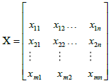
There are 19 indicators for decision-making and 5 options for decision-making in this research. Therefore, the decision-making matrix is X_7x21. Using the fuzzification scale, we converted the obtained qualitative data into triangular fuzzy numbers. The fuzzified decision matrix will be as presented in Table 16.

Defuzzification of the decision-making matrix

The decision-making matrix n is defuzzified in the second step. The fuzzy normal matrix is displayed with the symbol and each element of the normal matrix will also be displayed as . We use the following equation in order to normalize the data.

If the criterion has a negative charge, we will use the following equation:

All of the criteria are positive in this study. Date for the descaled fuzzy decision matrix is presented in Table 17.

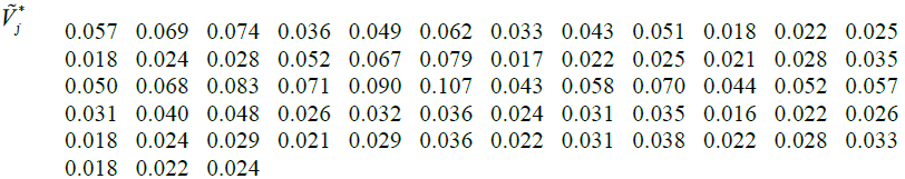
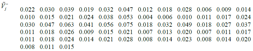
Fuzzy Weighted descaled Matrix

Fuzzy Weighted descaled Matrix should be formed in the third step (Table 18). This matrix is displayed with symbol . Having the weights of the indicators which are shown with the vector, we will have:

In general, the descaled matrix (N) should be converted into the weighted matrix (V). To obtain the weighted descaled matrix, we should have the weights of the indicators. The weight of each index has been calculated using the ANP technique in the following way

Having the weights of the indicators which are shown with the vector, we will have:

In the next step, the ideals for the positive and negative values should be calculated:

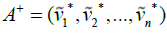
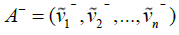
According to one view, is the best value of Criterion i among all of the options and is the worst value of Criterion i. i among all of the options. Since the normalized triangular fuzzy numbers belong to the range [0, 1], so the positive and negative ideals proposed by Chen (2000) are as follow:

The first approach is used in this study. So the values are as follows:

Ideal positive and negative calculation

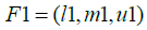
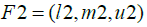
Given the values and positive and negative ideals can be calculated. Then, the total distance of options should be calculated from the positive and negative ideals. If F1 and F2 are two triangular fuzzy numbers, then the distance between these two numbers will be calculated as follows:

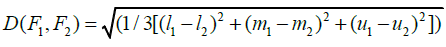
CL value is between zero and one. The closer this value is to one, the closer the solution is to the ideal answer, and it is a better solution. After calculating the unbalanced matrix, the distance of each option from the positive ideal and from the negative ideal has been calculated. The distance of each option from the ideal positive has been shown by D+ and the distance from the negative ideal has been displayed by D-. To calculate the ideal solution, the relative closeness of each option to the ideal solution is calculated. The closer the CL value is to one, the solution is closer to the ideal solution and it is a better solution. The TOPSIS computation output for these equations is in the form of Table 19.

So, given the calculated values shown in the table, it can be concluded that company D is the best option. E is also ranked second with a weight of 0.516.

Results & Discussion

The Results of the Main Criteria of the Research

The main criterion of the research was improving the sustainable supply chain performance by comparing the three economic, environmental, and infrastructural and cultural infrastructure factors and we concluded based on the analysis and the eigenvector that economic factors have the first priority with the normal weight of 0.437, the environmental factors have the second priority with the normal weight of 0.319, and the infrastructural and cultural factors have the last priority with the normal weight of 0.244. The reason for the higher priority of the economic factors than the infrastructural and cultural factors in the sustainable supply chain performance improvement can be due to the fact that cost of resources, production cost and supply chain cost are the sub-criteria of the economic cost.

The Results of the Sub-criteria of the Research

Economic sub-criteria

First, we have presented the calculations made to determine the priority of the economic sub-criteria. The economic sub-criteria include: automation, supply chain cost, cost of return, product durability, cost of design, cost of resources, production cost, and flexibility of supply. As this criterion consists of 8 indicators, so 28 pair-wise comparisons were made, and we came to the conclusion that the cost of resources index is of greatest importance with the normal weight of 0.208, the automation index has the second priority with the normal weight of 0.196, and the supply chain cost index has the third priority with the normal weight of 0.163. The researcher thinks that the reason for the high priority of the cost of resources index can be the fact that there will be no supply chain until the cost of the resources is not supplied and the cost of resources is actually the driving engine of the supply chain in economic areas.

Environmental sub-criteria

Environmental sub-criteria include: integration and participation, integration of processes, understanding the market disequilibrium, Dangerous factors of the workplace and community, and environmental pollution. As this criterion consists of 5 indicators, so 10 pair-wise comparisons were made, and we came to the conclusion that integration of processes is of greatest importance with the normal weight of 0.294, integration and participation has the second priority with the normal weight of 0.227, and understanding the market disequilibrium has the third priority with the normal weight of 0.191. The researcher thinks that the reason for the high priority of integration of processes can be the fact that supply chain includes production and reception of the product by customers. Therefore, the more ingrate the processes are, the more effectively and efficiently we will be able to have a sustainable supply chain.

Infrastructural and cultural sub-criteria

The infrastructural and cultural sub-criteria include: mutual trust and communication, timely and suitable delivery, quality improvement, rapid delivery, customers' status, humanitarian laws, performance of the business and marketing sectors, and culture and technology development. As this criterion consists of 8 indicators, so 28 pair-wise comparisons were made, and we came to the conclusion that mutual trust and communication is of greatest importance with the normal weight of 0.149, customers' status has the second priority with the normal weight of 0.142, and performance of the business and marketing sectors has the third priority with the normal weight of 0.139. The researcher thinks that mutual trust and communication can be the fact that since supply chain is defined in such a way that it covers the production stage and the time the product is purchased by customers, the greater and better mutual relationships between the buyer and the salesperson, the more sustainable supply chain and more improvement of sustainable supply chain performance we will have.

Conclusion

This research shows that several factors are effective in the success or improvement of supply chain performance. The first factor is the tom management's support of the process of organization's integration with suppliers and customers for the creation of supply chain. The second factor is people's (employees and managers) training which paves the way for new conditions in the organization. The third factor is effective and efficient information system for the effective and efficient flow of information in organizations, and this factor effectively helps the chain members to interact constructively. It may be said that the existence of a proper flow of information helps achieve many objectives of supply chain. In studies conducted on the most successful organizations in the implementation of supply chain management (Toyota, Dell, McDonald's, etc.), it has been shown that the management' support of the employees and individuals involved in supply chain and production and their commitment to customers contribute to the success of organizations. Training plays an important role in learning the new tasks and especially in making the employees multi-skilled in order to have personnel suitable for working in such organizations. Finally an information system that is based on accurate, timely and relevant information contributes to the profitability of the supply chain by eliminating a lot of waste and delay.

References

1. Alfat L., Seyyed Ali. K.F, & Allah A. (2011). Requirements for Implementation of Green Supply Chain Management in Iran's Automotive Industry, Journal of Management of Iran 6(21), 123-140.
2. Amin, S. H., Razmi, J., & Zhang, G. (2011). Supplier selection and order allocation based on fuzzy SWOT analysis and fuzzy linear programming. Expert Systems with Applications, 38(1), 334-342.
3. Amiri, M., Abadi. S.M.M, Shabani, A., & Mohammadi, K. (2009). An Analysis of Factors Affecting Supply Chain Performance with Fuzzy Approach Factor Analysis (Case Study: Shiraz Industrial Complex Industries). Scientific Supply Chain Management, 18 (54), 4-16.
4. Habibi, A., Sarafrazi, A., & Izadyar, S. (2014). Delphi technique theoretical framework in qualitative research. The International Journal of Engineering and Science, 3(4), 8-13.
5. Makui, A. (2000). Introduction to the Production Planning.
6. Nikpour, A., &  Salajegh. S. (2010). The relationship between organizational agility and job satisfaction among governmental organizations in Kerman, Management Research, 3 (7): 169-184.
7. Olfat, L., & Barati, M. (2012). An importance-performance analysis of supply chain relationships metrics in small and medium sized enterprises in automotive parts industry. Industrial Management Journal, 4(2), 21-42.
8. Park, J., Shin, K., Chang, T. W., & Park, J. (2010). An integrative framework for supplier relationship management. Industrial Management & Data Systems, 110(4), 495-515.
9. Porter, M.E., & Michael; ilustraciones Gibbs. (2001). Strategy and the Internet.
10. Rostamzadeh, R., Ghorabaee, M. K., Govindan, K., Esmaeili, A., & Nobar, H. B. K. (2018). Evaluation of sustainable supply chain risk management using an integrated fuzzy TOPSIS-CRITIC approach. Journal of cleaner production, 175, 651-669.
11. Sahebi., Z., Mottagi., & H Shojaee., M.R (2014). Applying the Fuzzy QFD Integrated Approach and TOPSIS in Choosing Supplier, Production and Operation Management, 6(2), 21-40.
12. Sharma, M. K., & Bhagwat, R. (2007). An integrated BSC-AHP approach for supply chain management evaluation. Measuring Business Excellence, 11(3), 57-68.
13. Teimoori, A. (2000). Developing the supplier selection model and distribution with chain management approach. Unpublished doctoral dissertation, Iran's University of Science and Technology.
14. Yu, W., Jacobs, M. A., Salisbury, W. D., & Enns, H. (2013). The effects of supply chain integration on customer satisfaction and financial performance: An organizational learning perspective. International Journal of Production Economics, 146(1), 346-358.