Introduction and Literature Review

Lag length selection is a generic problem in applied time series analysis. Many methods exist to avoid the ad hoc selection of lag length. Their performance is interesting because all statistical techniques depend sensitively on the satisfaction of their underlying assumptions - including the use of the correct lag length.

Trends are usually modeled either deterministically or stochastically. In finite samples, these approaches are nearly observationally equivalent to each other, and also to autoregressive processes with large positive roots. The low power of tests to distinguish these models reflects this problem. So, applied researchers are left with the question of how best to account for this ambiguity in the early stages of modelling.

This study examines the performance, in a Monte Carlo setting, of lag selection methodologies when stochastically trending variables are modeled in three plausible ways. One of these is more efficient than the others. The other two are representative of the type of misspecification that can easily arise in applied work due to the near observational equivalence of deterministic and stochastic trend specifications. The question of interest is which specification actually works best when you don’t know which one is correct.

This study adds to several threads in the literature. For forty years researchers have been comparing the performance of lag selection methods in Monte Carlo settings (see Geweke and Meese (1981); Lütkepohl (1985); Nickelsburg (1985); Holmes and Hutton (1988); Judge et al. (1988); Kilian (2001); Ivanov and Kilian (2005); Hacker and Hatemi (2008). In a second thread, researchers have begun to examine how lag selection methods perform when the model specification is unknown or incorrect (see Hatemi, 2003), Hacker and Hatemi-J [2008], and Lohmeyer, Palm, Reuvers, and Urbain [2019]). Lag selection is now featured in texts for applied macroeconomists (see Canova, 2011), has been incorporated into financial spreadsheets for classroom use (see Mustafa & Hatemi, 2020), is showing up in the literature of others fields (see Aho et al., 2014), and is being newly applied in the latest time series research (see Li & Kwok, 2021). This paper contributes with a Monte Carlo study of correctly vs. incorrectly specified models of trending time series, as are commonly found in economics and finance.

Lag Selection Methodologies

There are two distinct methodologies for selecting lag lengths. One (introduced by Theil, 1961) minimizes a selection criterion. The other is traditional, and uses conditional hypothesis testing (Hannan, 1970) suggested this method for lag selection, and it was recently examined in Hatemi and Hacker (2011). Both are based on estimating a variety of plausible models. By definition, at most one of those is correctly specified.

Ultimately one of those models is chosen for further analysis. Underfitting the lag length of that model will lead to biased and inconsistent parameter estimates, and may lead to serial correlation in the residuals. Alternatively, overfitting yields inefficient parameter estimates.

Criteria minimization begins with some maximum lag to consider L. Then L models of the following form are estimated:

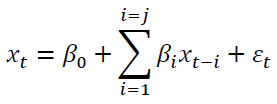(1)

Equation (1) may include other deterministic terms (including trends) without loss of generality. The index varies from 1 to L. From these regressions three values are obtained: N, the number of observations K, the number of right hand side variables, and , the estimated residual variance from the regression. The lag selected is the which yields the minimum from:

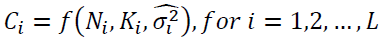(2)

Here Ci is one of the many selection criteria available in the literature. Some theory exists regarding the accuracy of this method (Akaike, 1974); Bhansali and Downham (1977); Hannan and Quinn (1979); Stone (1979); Geweke and Meese (1981), and shows that many of the potential functional forms are asymptotically equivalent.

Conditional hypothesis testing begins with a maximum lag , and a single estimate of (1) with j = L. Then a sequence of conditional nested hypothesis tests of the form 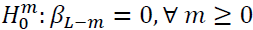, are made. The sequence begins with m = 0, and continues until a null hypotheses is rejected. Then the lag length for the model is set to (L-m+1). The asymptotic justification for this method is standard. However, a significance level α must be selected a priori, and this choice is not without a further potential pitfall.

Many studies (cited above) examine these methodologies in finite samples. They demonstrate that the methods do differ, and that they can be roughly ordered from least to most parsimonious. Further, there is a consensus that all the methods are more likely to underfit the true lag when conditions are less than ideal. The sensitivity of selection criteria to the true trend process, and to how it is modeled is not known asymptotically or in finite samples. However, it is known (Sims et al., 1990) that the conditional tests described above will often have standard distributions. In fact, the only test that will have a non-standard distribution (in the single unit root case) is the very last test that all L lags are jointly zero.

The Monte Carlo Experiment

Five methods for lag length selection are reported in a Monte Carlo simulation. Three are based on selection criteria, and two are based on hypothesis tests. The selection criteria are Theil’s (1961) residual variance criterion (RVC), Akaike’s (1974) information criterion (AIC), and Schwarz’s (1978) criterion. The hypothesis test methods are based on the likelihood ratio test (suggested in Hannan, 1970) with a significance level of either 5% or 1% (to account for Anderson’s suggestion). RVC is the oldest criterion, and has some similarity to adjust R². AIC and SBC are representative of the family of criterion available in econometrics textbooks. Hannan’s methodology is representative of the sequential testing methodology often used in VAR analysis (as suggested in Sims 1980).

In each Monte Carlo simulation, the data generating process shown in the tables below is an ARI (2,1) with drift: that is, a stochastic trend. The drift is held constant at one. Thus, changing the residual variance of the data amounts to changing the proportions of sample variance that result from the residual and the stochastic trend. The variance of the residual is either large (10) or small (1). The autoregressive roots are always held equal to each other, and are either large (0.9) or small (0.1). Thus, the generated data displays persistence due to the positive roots. These setups are typical of economic and financial data.

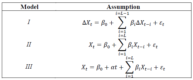
Two alternative modeling assumptions are made prior to the lag selection. In the first, the researcher is presumed to know that the series in question is integrated, and is thus working with the differences. Since this restriction is true, this assumption is the most efficient. Critically, applied researchers usually do not know this specification is correct at the time they do their lag selection. The second assumption is that the researcher does not know the processes are integrated, and therefore models them in one of two ways: in levels either with or without a trend term. The two versions of this method will be inefficient relative to the first method since it estimates the unit root as a free parameter, and may include an irrelevant regressor. This yields three model assumptions.

Each of the model assumptions is readily familiar to applier researchers. Importantly, at the time that the applied researcher does their lag length selection, they do not know which model is correct. Given the data generating process for the Monte Carlo simulation, I is always correct in this study. This is also the null hypothesis of typical unit root tests, where II and III are the regressions commonly used at the start of research papers that justify going forward with I for results reported towards the end of research papers. It is ironic that the properties of lag selection criteria have never been examined for this common situation.

All three models share the small degree of bias associated with estimating auto regressions in finite samples. The correct lag is two in I and three in the other ones.

In sum, the simulations examine 5 methods for lag selection, for 3 different assumptions about the model used, for 4 varieties of data generating process. One million simulations are run for each of those 60 cases. Percentages are rounded, and occasionally below, dominance is reported although digits confirming that were rounded off.

Results

Each of the tables reports the results of five alternative methods for lag selection. Three are selection criteria. RVC is the classic heuristic that lacks parsimony. Akaikie’s and Schwarz’s criteria (AIC and SBC) are grouped together since they share a more formal theoretical justification, but are known to be more and most parsimonious in finite samples. Lastly hypothesis tests using a likelihood ratio statistic are grouped together, with a larger and smaller significance level examined for less and more parsimony. The percentages of simulations that were underfit, correctly fit, and overfit are reported.

The goal here is to find a modeling assumption that dominates another one, in the sense that it both underfits and overfits less (and therefore also yields the correct fit most often). Where possible, the three model assumptions are ranked. This is shown in its own column. A weaker secondary goal, because it can be achieved by either underfitting or overfitting less, is to find the modeling assumption that merely leads to the correct lag length the most. This is marked by an asterisk.

Table 1 reports results when the selection methods should have an easy time of it. The autoregressive roots in the data generating process are large. The residual variance that might confuse the methods is small. This corresponds to a series that, when plotted, trends but is quite smooth; perhaps something likes a price level.

Table 1 Results when Autoregressive Roots are Large and Residual Variance is Small Data Generating Process:
	Optimal				%	%	%
Criterion	Model	Lag	d	t	Underfit	Correct Fit	Overfit	Rank
RVC	I	2	1	0	0	38.9	61.1
RVC	II	3	0	0	0.1	84.5*	15.4	II > III
RVC	III	3	0	1	0.3	79.5	20.2
AIC	I	2	1	0	0	72.2	27.8
AIC	II	3	0	0	0.1	90.6*	9.3	II > III
AIC	III	3	0	1	0.3	85.4	14.3
SBC	I	2	1	0	0	96.0	4.0	I > III
SBC	II	3	0	0	0.1	96.8*	3.1	II > III
SBC	III	3	0	1	0.5	93.1	6.4
LR, α = .05	I	2	1	0	0	89.1*	10.9
LR, α = .05	II	3	0	0	46.0	53.0	1.0	II > III
LR, α = .05	III	3	0	1	58.5	40.4	1.1
LR, α = .01	I	2	1	0	0	97.8*	2.2
LR, α = .01	II	3	0	0	53.1	46.7	0.2	II > III
LR, α = .01	III	3	0	1	64.7	35.1	0.2

Initially, the performance of the methods is examined. This helps show consistency with the existing literature.

As expected, when comparing the 3 criteria methods, RVC is the least parsimonious. It overfits more for all 3 models. AIC and SBC do better. They overfit less, without underfitting much more.

The hypothesis tests do far worse. They underfit about half the time in the two levels specifications. LR with low significance level is the most parsimonious. The most glaring result is that conditional hypothesis testing on a levels specification will miss at least one large autoregressive root over half the time. This does not occur when the data is differenced. That is problematic since differencing is generally the researcher’s conclusion, and not their position when doing initial work. This is bothersome, since Anderson’s (1971) suggestion is sensible, but appears to be too much of a good thing.

What makes this paper different is the focus on model specification when the true data generating process is unknown. Looking at the ranks, we can see that for 4 of the 5 situations, II strictly dominates III. This is an important result for unit root testing, where one can either exclude or include the trend term (as in II and III), but where there is little justification for going either route. Readers may be surprised at this: there is little theoretical reason to expect any pattern of dominance whatsoever.

There is no clear dominance between the levels specifications and the differenced specification. Having said that, many researchers will look at these results and prefer to stick with levels when using selection criteria, since over fitting is the more common problem and can be mitigated. Nonetheless, readers should be surprised at this as well:

The theoretically correct model, and the one for which estimation will be more efficient, did not dominate the others.

Alternatively, if the researcher is inclined to use hypothesis testing, then the opposite conclusion follows. Here underfitting is the bigger problem, and it can be mitigated by choosing to difference.

This is also the first evidence of an interesting insight of these simulations. The 3 selection criteria tend to perform better with the mildly misspecified model II. The 2 hypothesis tests perform better when the model is correctly specified, as in I. Of course, that’s problematic since the true data generating process is generally unknown.

There is also evidence of a central insight for practitioners. They often agonize over the choice of selection method that will best display their desired conclusions. But an examination of Table 1 shows there really isn’t any dominance of one of the five methods over another: each is capable of underfitting or overfitting a bit worse than its competitors. For example, SBC clearly overfits less, but it isn’t clear that it underfits less as well. This suggests that researchers’ concerns about the choice of criteria may be less important than their choice of model.

To some it may be easy to dismiss this concern, but we should not. Table 1 demonstrates a pattern that shows up in the later tables too. The choice of selection criteria that applied researchers often agonize over is between the blocks of three rows in the table. Consider a researcher who has settled on model II. The magnitude of the difference they are worried about between, say, RVC and AIC is about 6%. Yet this is comparable to the 5% difference between choosing models II or III with either criterion, and far smaller than the differences between choosing model I. This suggests that the choice of model is at least as important as the choice of criterion.

Table 2 reports the results with identical autoregressive roots, but with a larger residual variance. This corresponds to a series that, when plotted, trends but can have extended swings above and below trend; perhaps something like real GDP.

Table 2 Results when Autoregressive Roots are Large and Residual Variance is Large Data Generating Process:
	Optimal				%	%	%
Criterion	Model	Lag	d	t	Underfit	Correct Fit	Overfit	Rank
RVC	I	2	1	0	0	38.9	61.1
RVC	II	3	0	0	0	41.7*	58.3	II > I,III
RVC	III	3	0	1	0	40.0	60.0	III > I
AIC	I	2	1	0	0	72.2*	27.8	I > II, III
AIC	II	3	0	0	0	71.6	28.4	II > III
AIC	III	3	0	1	0	69.5	30.5
SBC	I	2	1	0	0	96.0*	4.0	I > II, III
SBC	II	3	0	0	0	95.6	4.4	II > III
SBC	III	3	0	1	0	94.7	5.3
LR, α = .05	I	2	1	0	0	89.1	10.9
LR, α = .05	II	3	0	0	0	89.2*	10.8
LR, α = .05	III	3	0	1	0	87.8	12.2
LR, α = .01	I	2	1	0	0	97.8*	2.2
LR, α = .01	II	3	0	0	0	97.7	2.3
LR, α = .01	III	3	0	1	0	97.1	2.9

The performance of RVC is worse in this case. Overfitting is more common. AIC also tends to perform worse; however, SBC is not fooled much by the higher residual variance.

For the hypothesis tests, underfitting has been eliminated, and overfitting is quite modest. This harkens to something a bit like multicollinearity: in Table 1 there isn’t enough residual variance for a hypothesis test to delineate the autoregressive roots well, but the larger variance in Table 2 helps them both stand out as important. While not the main focus of this paper, this is a novel result.

As to the rankings, which are an important implication of this paper, there is no firm conclusion. Model II dominates III in a majority of the cases. But, model I performs better in Table 2 than in Table 1. Having said that, all of the models are so close that it seems in this case that the choice of selection criteria is more important than the choice of model. Models I and II split the results for the weaker criteria of most correct fits.

Table 3 reports the results of simulations where both the autoregressive roots and the residual variance are small. Because of the interaction of autoregressive roots and residual variance in time series models, this is the data generating process that will be the smoothest, with little persistence to shocks, and little variation around the trend; perhaps something like real household consumption.

Table 3 Results when Autoregressive Roots are Small and Residual Variance is Small Data Generating Process:
	Optimal				%	%	%
Criterion	Model	Lag	d	t	Underfit	Correct Fit	Overfit	Rank
RVC	I	2	1	0	37.3	12.3	50.4
RVC	II	3	0	0	38.8	13.4*	47.8	II > III
RVC	III	3	0	1	39.1	12.5	48.4
AIC	I	2	1	0	74.2	10.9	14.9
AIC	II	3	0	0	73.3	11.5*	15.2
AIC	III	3	0	1	73.2	10.3	16.5
SBC	I	2	1	0	97.3	2.2	0.5
SBC	II	3	0	0	97.1	2.4*	0.5	II > I
SBC	III	3	0	1	97.0	2.2	0.8
LR, α = .05	I	2	1	0	88.8	0.8	10.4
LR, α = .05	II	3	0	0	88.4	1.1*	10.5
LR, α = .05	III	3	0	1	88.1	0.8	11.1
LR, α = .01	I	2	1	0	97.7	0.2	2.1
LR, α = .01	II	3	0	0	97.5	0.3*	2.2
LR, α = .01	III	3	0	1	97.4	0.2	2.4

Given the much weaker autoregressive components, all of the criteria have a tougher time with accurate selection. Underfitting is way up for each of the methods, and is almost certain when using SBC or hypothesis testing with a low alpha.

There is less evidence of dominance between the models here, but there is some. In both case, II is dominant. On a somewhat weaker note, for researchers who are most interested in a precisely correct fit, II is the unanimous choice.

Table 4 reports results with the same weak autoregressive roots as in in Table 3, but with a larger residual variance. Astute readers will note that the combination of lower root and higher residual variance makes the overall variance of X in Table 4 identical to that in Table 1. This is intentional and points out to downstream users that it isn’t the variance of the variable that delineates behavior, but rather the residual variance from the regressions.

Table 4 Results when Autoregressive Roots are Small and Residual Variance is Large Data Generating Process:
	Optimal				%	%	%
Criterion	Model	Lag	d	t	Underfit	Correct Fit	Overfit	Rank
RVC	I	2	1	0	37.4	12.3	50.3
RVC	II	3	0	0	40.3	13.1*	46.6
RVC	III	3	0	1	39.1	12.5	48.4
AIC	I	2	1	0	74.2	10.9*	14.9
AIC	II	3	0	0	74.7	10.6	14.7
AIC	III	3	0	1	73.2	10.3	16.5
SBC	I	2	1	0	97.3	2.2	0.5
SBC	II	3	0	0	97.3	2.1	0.6
SBC	III	3	0	1	97.0	2.2*	0.8
LR, α = .05	I	2	1	0	88.8	0.8	10.4
LR, α = .05	II	3	0	0	89.2	0.9*	9.9
LR, α = .05	III	3	0	1	88.1	0.8	11.1
LR, α = .01	I	2	1	0	97.7	0.2	2.1
LR, α = .01	II	3	0	0	97.7	0.2	2.1	II > I
LR, α = .01	III	3	0	1	97.4	0.2*	2.4

Once again, there is little evidence of dominance in the scenario with smaller roots. When it is there II is dominant. And by the weaker criteria of which model tends to produce the most correct fits, II wins in 3 of five.

Contrasting all four tables suggests five implications about the performance of the five selection methods:

1) There is little reason to expect any dominance at all between the three models. And yet II dominates quite often.

2) Mostly II dominates III. This is important since there are different “flavors” of unit root test, which either include or exclude a trend term. There is little theoretical reason to choose between them, but here there is a finite sample reason.

3) The selection criteria perform best in II. In two thirds of cases it yields the correct fit the most often (an unusual result with three possible models).

4) In many cases, the choice of model leads to larger differences between specific criterions, than the choice between the criteria themselves.

5) Otherwise, the performance of the simulations is consistent with earlier work: large autoregressive roots are easier to detect, RVC is least parsimonious, SBC is most parsimonious, etc.

These results suggest an interesting methodology. While most economic analysis presumes unit roots are in the data, these results suggest that this should not be imposed for lag length selection. In short, use a mildly incorrect model at this stage.

Conclusion

The performance of lag selection methodologies when the true process has a unit root is investigated. Additionally, the researcher may have mistaken the unit root process for the nearly observationally equivalent deterministic trend process. Many applications (e.g. unit root tests) require the specification of a lag structure when the true trend structure is unknown. Hall [1994] was the first to show that unit root tests perform better when lag selection methodologies are used prior to the actual test. However, he assumed that the researcher knew a priori that the true trend process was a unit root when choosing the lag length. This is unlikely, and a more realistic situation is examined here.

Imposing the correct assumption delivers the best performance only when both the autoregressive roots and the residual variance are large. This is also the data generating process that performs the best for all of the methods. We suggest that this is an unusual characterization of most data generating processes.

The likelihood ratio tests perform very poorly relative to selection criteria when the autoregressive roots are large, and variance is small. This suggests that some care must be taken in applying this method to smooth series such as price indices.

Imposing the (true) unit root restriction, even though this will increase efficiency, does not improve the performance of either the criteria, or the likelihood ratio tests. Further, there is never a large loss in the percent of correct fits when an incorrect model is estimated, and often a gain when the model is estimated in levels without a trend. Why is this so? A conjecture is because efficiency is a qualitative statement about estimation, while lag selection is a comparative process in which the qualitative failings of a particular model may wash out.

In the absence of further evidence these results suggest that lag selection should always be done with the data in levels, even if a unit root is suspected. Further, there is little to lose by adding a deterministic trend to the model, even when this assumption is false. This suggests the need for a parallel examination of the performance of models with deterministic trends when these may be misspecified.

References

1. Aho, K., Derryberry, D., & Peterson, T. (2014). Model Selection for Ecologists: The Worldview of AIC and BIC. Ecology, 95, 631-6.
2. Akaike, H. (1974). A new look at the statistical model identification. IEEE transactions on automatic control, 19(6), 716-723.
3. Anderson, T.W. (1971). The Statistical Analysis of Time Series, Wiley: New York.
4. Bhansali, R.J., & Downham, D.Y. (1977). Some Properties of the Order of an Autoregressive Model Selected by a Generalization of Akaike’s EPF Criterion.  Biometrika, 64, 547-51,
5. Canova, F. (2011). Methods of Applied Macroeconomics Research. Princeton University Press.
6. Geweke, J., & Meese, R. (1981). Estimating regression models of finite but unknown order. International Economic Review, Pp. 55-70.
7. Hacker, R., & Hatemi-J, A. (2008). Optimal lag-length choice in stable and unstable VAR models under situations of homoscedasticity and ARCH. Journal of Applied Statistics, 35(6), 601-615.
8. Hall & Alistair (1994). Testing for a Unit Root in Time Series with Pretest Data-Based Model Selection," Journal of Business and Economics Statistics, 12, 461-70.
9. Hannan, E.J. (1970). Multiple Time Series. Wiley: New York.
10. Hannan, E.J., & Quinn, B.G. (1979). The Determinants of the Order of an Autoregression. Journal of the Royal Statistical Society, B41, 190-5.
11. Hatemi-J, A., & Hacker, R.S. (2011). Can the LR Test Be Helpful in Choosing the Optimal Lag Order In the VAR Model When Information Criteria Suggest Different Lag Orders. Applied Economics, 41, 1121-1125.
12. Hatemi-J, A. (2003). A New Method to Choose Optimal Lag Order in Stable and Unstable VAR Models, Applied Economics Letters, 10, 135-7.
13. Holmes, James M., Hutton, & Patricia, A. (1989). Optimal’ Model Selection when the True Relationship is Weak and Occurs with a Delay, Economics Letters, 30, 333-9.
14. Ivanov V., & Kilian, L. (2005). A Practitioner’s Guide to Lag Order Selection for VAR Impulse Response Analysis,” Studies in Nonlinear Dynamics and Econometrics, 9.
15. Judge, G.G., Hill, R.C., Griffiths, W.E., Lütkepohl, H., & Lee, T.C. (1988). Introduction to the Theory and Practice of Econometrics, J. Wiley.
16. Kilian, & Lutz. (2001). Impulse Response Analysis in Vector Autoregressions with Unknown Lag Order. Journal of Forecasting, 20(3), 161-179.
17. Li, N., & Kwok, S.S. (2021). Jointly determining the state dimension and lag order for Markov‐switching vector autoregressive models. Journal of Time Series Analysis.
18. Lohmeyer, J., Palm, F. Reuvers, H., & Urbain, J.P. (2019) Focused Information Criterion for Locally Misspecified Vector Autoregressive Models. Econometric Reviews, 38(7),763-792.
19. Lütkepohl & Helmut. (1985). Comparison of Criteria for Estimating the Order of a Vector Autoregressive Process. Journal of Time Series Analysis, 6, 35-52.
20. Mustafa, A., & Hatemi J. (2020). A VBA module simulation for finding optimal lag order in time series models and its use on teaching financial data computation. Applied Computing and Informatics.
21. Nickelsburg, G. (1985). Small-sample properties of dimensionality statistics for fitting VAR models to aggregate economic data: A Monte Carlo study. Journal of Econometrics, 28(2), 183-192.
22. Schwarz, G., (1978). Estimating the Dimension of a Model. Annals of Statistics, 6, 461-4.
23. Sims & Christopher A., (1980). Macroeconomics and Reality. Econometrica, 48, 1-48.
24. Sims, Christopher A., Stock James, H., Watson, & Mark, W. (1990). Inference in Linear Time Series Models with Some Unit Roots. Econometrica, 58, 113-44.
25. Stone, M. (1979). Comments on Model Selection Criteria of Akaike and Schwarz. Journal of the Royal Statistical Society, B41, 276-8.
26. Theil & Henri, (1961).  Economic Forecasts and Policy, North-Holland: Amsterdam.