Keywords

Modeling, Services, Revenue Optimization, Customer Service, Loyalty.

Introduction

Many customer experiences combine a longer term view of the customer from services and the more traditional margin-based approach on product sales. Many companies are now focusing on services revenues (Allen 2020). Cars are big business (Wikipedia, n.d.).

Literature Review

If one considers the potential the impacts of waiting, in this case while service is completed, research suggests that the effect of waiting is equivocal. On the one hand, discounted utility theory (Loewenstein & Prelec 1992) would predict that wait times are negative, and consumers prefer quicker service. On the other hand, consumers may derive utility from anticipating an experience (Caplin & Leahy 2001; Moller & Erdal, 2003). Nowlis et al. (2003) reconciles these two seemingly opposing points of view, making it an exercise without utility to address such questions here.  However, many firms are trying to balance the time a customer spends waiting with their potential to think of items they might want to purchase during said wait time. For instance, such time can be used to decide that one decides a vehicle would be a smart purchase. In this sense, the showroom becomes a waiting room. To complete the analogy, magazines are replaced with inventory. Figure 1 depicts this relationship. The remaining paper uses modelling to predict how such wait times impact overall profitability, including those from service (that benefit from lower wait times) and those from sales of goods (that benefit from longer wait times) (Chen et al., 2007).

Methodology 

Let p be the profit a dealership receives (note: for a summary of all variables, see Table 1 in the Appendix). This is combined of two values: x, which is the expected future cash flows of service margin due to a satisfied customer, and y, which is the expected margin received from selling a car to someone who is made to hang around a dealership while the service personnel slow down the rate of service (Marrewijk, 2003; Smith, 2003).

(1) X + y = p

Let a be the function of the difference between the estimated time of service and the actual time of service, acting as referent point for the customer. Or, more formally:

(2) a*x + y = p

Let a² be the function of the length of time over the time period that is two times the expected length, because it’s quadratic and people get really mad when it takes that long.

(3) a*a²*x + y = p

Let b be the expected life of a the car, which is a function of c which is how many miles over 100,000 are on the car.

(4) a*a²*x*b(b-c) + y = p, or

(5) a*a²*x*b²-bc + y = p

Let d represent the quality of the waiting room amenities. Plus one if there is coffee.

(6) ((a*a²*x*b²-bc)d+1) + y = p

Let e represent the alignment of the gender between the customer and the service agent, represented as -1 if they are both female, +1 if they are both male, and 0 otherwise.

(7) (((a*a²*x*b²-bc)d+1)e) + y = p

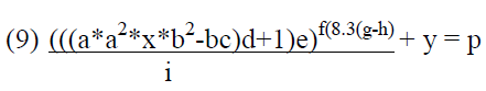
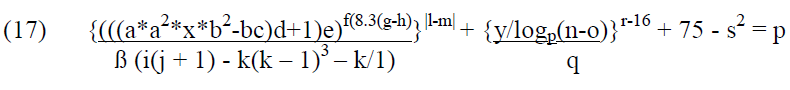
Let f represent the period of time lapsed, in hours, since the customer has last eaten; further, 8.3(h-g) indicates that g is the caloric intake of the last meal, and h is the BMI of the customer. Or, more formally:

(8) (((a*a²*x*b²-bc)d+1)e)^f(8.3(g-h) + y = p

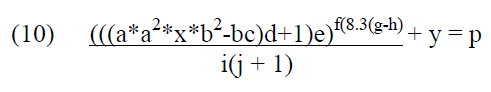
Let i represent the number of times the customer has previously had their vehicle serviced at this particular establishment:

Let j+1 represent the previous number of vehicles the customer had serviced at this particular establishment:

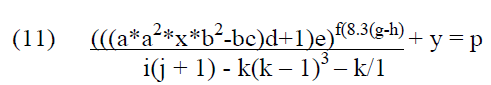
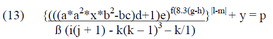
Let ?k represent the change in ambient natural light emitted into the area where the customer is waiting, or ?k = k(k – 1)³ – k/1. Or, more formally:

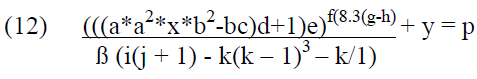
 Let ß represent the rate of speed the car makes as it pulls around into the parking space. Just because.

Let l represent the difference between the price paid from the monthly budget, m, of the customer over and above the cost of rent.

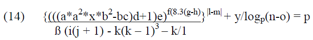
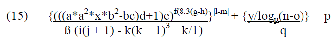
The n represent the proximity of the date of the year of manufacture of the new car, relative to the year in which the customer was 16 years of age, represented by o. In order to compensate for musical genre effects, take a log of the difference to the base of the number of cassette tapes in the customer’s first car, or p. More formally: 

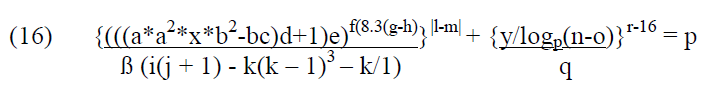
Let q represent the ground clearance of the new vehicle. Lower vehicles are cool.

 Let r represent the rim size of the wheels on the vehicle purchased.

The variable s represents the BMI of the sales person, with a theoretical maximum of 75.

 Let t represent the finance rate of the new vehicle, financed at an outstanding balance of u, expressed as NPV.

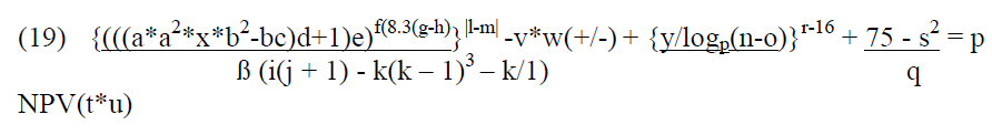
 Going back to the service environment, adjusting for the number of children present during the visit, v, and the overall length of time spent in the showroom, w, we calculate a propensity of purchase with is a function both positively and negatively affected by v and w.

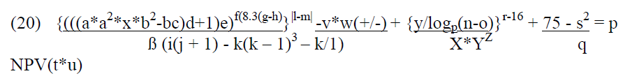
 However, if there is a nursery-like play area in the showroom area, based on the type of lettered blocks including X, Y and Z, we calculate:

Results and Discussion

As is evident from the final, fully developed model, the optimal level of profitability is a combination of potential profit from both services and goods (Hood et al., 2013). The revenue from each of these two streams must be optimized in order to get big bucks. Many managers seek to acquire bonuses that are based on profit acquisition. Therefore, the application of these rules can have a positive impact on the career of managers who implements such policies. Constraints and limitations are inherent in the model. Cultural differences around the global may necessitate the customization of this model. For example, local training should embrace cultural differences in learning, and local customer value should be considered in both services and goods (Fuentes & Rojas, 2001).

Conclusions and Future Considerations

Future research can empirically test the models presented here. Each of the items here can be considered, very carefully, by both academicians and practitioners. Practitioners are the stakeholder that will implement the ideas; academicians are responsible for further testing and model refinement.

Appendix

Table 1 Directory of Modelled Variables
Variable	Definition	Measurement
Profit (p)	The surplus that remains once expenses have been deducted from revenues.	Dollars, pesos, euros, yen or Bitcoin.
Service cash flows (x)	The net present value (discount rate applicable) from future revenues from servicing a vehicle, present and future, for a given customer.	Individual level variable, per customer, measured in the same denomination as profit.
Margin from sales of goods (y)	Surplus revenue after expenses from the sale of a vehicle. Does not include undercoating.	Same as x.
Perceived wait time (a)	Difference between expected wait time and actual wait time.	Individual level variable, measured in minutes in a weekday, hour on a weekend.
Expected lifetime use (b)	The expected lifetime value of a vehicle.	Individual level variables, measured in years.
Quantification of long life (c)	Total vehicle mileage, less 100,000 (zero if mileage is < 100,000).	Measured in miles if USA, kilometers in other cultures requires multiple of 1.6.
Service-related Amenities (d)	Perceptual score, based on surveys, of the quality of amenities. Limited to those inside a physical structure.	Individual level variables, likert scale from 1 (poor) to 7 (excellent).
Gender alignment (e)	Alignment of the gender between the customer and the service agent.	Individual level variable: -1 if they are both female, +1 if they are both male, and 0 otherwise.
Time since eating (f)	Time lapsed since last eating.	Individual level variable. Measured in hours.
Caloric content (g)	Density of consumption.	Individual level variable. Calories (kilojoule conversion required in the customary fashion).
Body mass index (h)	Relationship between height and weight of the consumer.	Individual level variable. Measured in the customary fashion.
Current service history frequency (i)	Number of times a specific customer has sought service.	Individual level variable. Denoted with Arabic numerals.
Past service vehicle history (j)	Number of previous goods serviced at a given establishment.	Individual level variable. Denoted with Arabic numerals.
Ambient light (atmospherics (k))	Degree of natural light in an ambient environment.	Establishment level variable. Measured in lumens.
Speed at arrival (ß)	Speed of customer arrival.	Individual level variable. Measured in miles per hour if in USA, otherwise converted to kilometers in the same manner as vehicle life.
Budget parameters (l and m)	Monthly budget, after-tax, for a customer. Difference is the surplus, after the cost of service and rent, have been deducted from the budget.	Same as profit.
Date of vehicle manufacture (n)	The proximity of the date of the year of manufacture of the new car.	Individual level variable. Measured in years.
Customer age proxy	The calendar year in which the customer was 16 years of age.	Individual level variable. Measured using Gregorian calendar.
Customer cultural proxy (p)	The degree to which a customer’s musical preference will predict if they will be chill.	Individual level variable. The number of cassette tapes in the customer’s first car. Measured in the customary fashion.
Customer vehicular cultural proxy1 (q)	The degree to which a customer uses a vehicle for a optical form of cultural status.	Individual level variable. Measured in inches of ground clearance to lowest point of vehicle.
Customer vehicular cultural proxy2 (r)	The degree to which a customer uses a vehicle for a proportional form of cultural status.	Individual level variable. Wheel rim size, measured in inches.
Salesperson dimensions (s)	Body mass index of the salesperson.	Individual level variable. Measured in the customary fashion.
Financing rate (t)	The cost of financing used to purchase a good.	Individual level variable. Measured as a percentage.
Outstanding loan balance (u)	The balance of a borrowed sum at a given point in time.	Individual level variable. Measured like profit, expressed as an NPV.
Customer Distraction (v)	Degree to which a customer will be distracted by parenting demands.	Individual level variable. Measured by the number of individuals under the age of 18 with the customer in the establishment.
Length of service encounter (w)	The total time spent waiting for service completion.	Individual level variable. Measured in minutes during weekdays, hours on weekends.
Distraction compensatory potential (X, Y, Z)	The presence of an environment that can mitigate parental distraction (noted in v).	Individual level variable. Binary (1=yes, 0=no), based on presence of X, Y, and Z blocks in compensatory area.

References

1. Allen, A. (2020). Personal communication.
2. Caplin, A., & Leahy, J. (2001). Psychological Expected Utility Theory and Anticipatory Feelings. Quarterly Journal of Economics, 116, 55-79.
3. Chen, M.H., Jang, S.S., & Kim, W.G. (2007). The impact of the SARS outbreak on Taiwanese hotel stock performance: an event-study approach. International Journal of Hospitality Management, 26(1), 200-212.
4. Fuentes, N., & Rojas, M. (2001). Economic theory and subjective well-being: Mexico. Social Indicators Research, 53(3), 289-314.
5. Hood, M., Kamesaka, A., Nofsinger, J., & Tamura, T. (2013). Investor response to a natural disaster: Evidence from Japan's 2011 earthquake. Pacific-Basin Finance Journal, 25, 240-252.
6. Loewenstein, G., & Prelec, D. (1992). Anomolies in Intertemporal Choice: Evidence and an Interpretation. Quarterly Journal of Economics, 107, 573-597.
7. Marrewijk, M. (2003). Concepts and definitions of CSR and corporate sustainability: Between agency and communion. Journal of Business Ethics, 44(2-3), 95-105.
8. Moller, K., & Erdal, T. (2003). Corporate responsibility towards society: A local perspective. Dublin: European Foundation for the Improvement of Living and Working Conditions.
9. Nowlis, S., Mandel, N., & McCabe, D.B. (2003). The Effect of a Delay Between Choice and Consumption on Consumption Enjoyment. Journal of Consumer Research, 31, 502-510.
10. Smith, N.C. (2003). Corporate social responsibility: whether or how?. California Management Review, 45(4), 52-76.