Research Article: 2020 Vol: 21 Issue: 3
Oil Price Overshooting, Monetary Policy and Economic Activity: Evidence from Oil Producing Nations
Ebenezer Adesoji Olubiyi, Federal University of Agriculture, Nigeria
Eunice Oluganna, Federal University of Agriculture, Nigeria
Abstract
This study focuses on the time adjustment paths of the oil price, industrial price and exchange rate in response to unanticipated monetary shocks in the oil producing countries. The basic Dornbusch model of overshooting was modified to include oil and industrial prices and then investigate the influence of this overshooting on economic activity. Annual data spanning 1991 to 2018 were extracted and Johansen’s cointegration test alongside a panel vector error correction model is employed to investigate the overshooting using the error correction terms of the variables. The empirical results indicate that all these prices overshoot their long run equilibrium. Oil price adjust faster to its long run equilibrium than exchange rate following innovations in the money supply. Vector error correction Granger Causality/Block Exogeneity Wald Tests is used to test for dynamic causality between the variables. Causation runs from money supply to oil price and GDP. GDP causes oil price as well. Further, oil price causes industrial prices and effective exchange rate. Also, Impulse response functions and Variance decompositions is used to show the effects of shocks on the adjustment path of the variables in the panel VECM model. Policy implications and recommendations are proffered based on these findings.
Keywords
Oil Price Overshooting, Exchange Rates, Economic Activity, Monetary Shocks, Panel Vector Error Correction.
JEL Classifications
Q21, F31, E32, E20, C33.
Introduction
Oil has been an important factor input in most economies of the world but not all countries are endowed with it. Consequently, the commodity has become one of the most traded in the world market. By implication, most governments of countries endowed with oil, depend heavily on the revenue generated from the proceeds. In particular, the Organization of Petroleum Economic Community (OPEC) and some non-OPEC members rely mostly on oil proceeds as a means of propelling their economies (Olubiyi & Olopade, 2018; Olubiyi, 2019).
However, owing to persistent unstable price of oil, the growth time-path of these countries appear to be unstable. Oil price fluctuation is caused by shifts in demand for oil and the political events. The shift in demand is further caused by continuous global discovery of technological breakthrough that is oil-dependent and also the demand for oil inventories in other to safeguard future shortages (Areszki, et al. 2017). Aside from the demand shift, another major cause of oil price fluctuation is political events and economic policy of the monetary authorities. The first noticeable oil price shock occur in 1973 when the Arab oil producing countries and members of OPEC placed embargo on the supply of oil in response to the Yom Kippur war (Caraiani & Calin, 2019). Oil price rose from its pre-1973 stable price of $20 to $40. In the 1980s, oil price experienced downward trend owing to war between Iran and Iraq.
Towards the end of 1980, major oil producing countries embarked on oil conservation and insulation and this caused the price of oil to drop to $22. But in 1990, the Persian Gulf War (PGW) which led to the contraction of oil production and, by implication, oil price spiked to $65. This price could not be maintained due to Asian financial crisis, which led to low demand for oil forcing a downward trend to an average of $15. Perhaps oil price could have hovered around this price for a relatively long time if not for a security threat against the US economy by the Terrorists in September 2001 that caused oil price to rose as much as $45. During the US-led Iraq invasion, oil price jumped to $80 while the Middle East tension and industrial revolution of China, caused all oil price to rise as high as $103.97 (Gaidar, 2007). Russia, a major non-OPEC oil producing nation and Saudi Arabia, a major OPEC oil producing nation flooded the oil market in the 2014-2015 period (Smith et al. 2015). During this period, China also experienced economic downturn that necessitated low demand for oil. All these led to supply shock and consequently forced oil price to go as low as $30. But due to economic stability and the fact that the Chinese economy is picking up, oil price rose gradually from $32 in 2016 to $53.07 in 2017 and further to $70.37 in 2018. As the US planned to respond to Dowing Chemical Attack in Syrian Civil War, oil price rose slightly to $72.04 and since the OPEC announced that oil production will be kept low, oil price grew gradually to $77.5 in 2019 and by February 2020 and March 2020, oil price dropped to $53.27 and $34 respectively owing to the outbreak of Coronavirus (COVID-19) which disrupts economic activity in countries with high demand fpr crude oil,
From the ongoing, it is clear that oil price has been volatile, suggesting that there are relevant information in it. One of such information is the monetary policy reaction to economic behavior. During the period of high oil price, aggregate price level will rise for at least two reasons. First, crude oil price is part of this aggregate price level and the price of goods for which crude oil serve as input will also rise. Also, if the cost of producing crude oil is high, the price will be on the high side. Among the oil producing countries, cost of production is low in Saudi Arabia, Iran and Iraq but the cost of production is high in Brazil, Nigeria and the United Kingdom. So, increase in aggregate price triggers inflation and this is where the monetary authorities intervene because the major function of the monetary policy is to keep inflation as low as possible. In the process of stemming inflation, oil price tends to overreact, that is, oil price overshoots its long run price due to monetary intervention.
Oil price overshooting may be more pronounced in the countries where oil proceeds are the mainstay. In this case, increase in oil price leads to more oil revenue and so aggregate demand will rise. Increase in aggregate demand leads to increase in inflation rate and this causes monetary authority to react by decreasing money supply. Decrease in money supply makes the purchase of imported raw materials and consumer goods to rise due to rising relative price and appreciation of exchange rate. In effect, the cost of production increases and the price level of final goods and services also increase, leading to inflation. Hence, there appears to be a link between oil prices overshooting, monetary policy and economic growth in oil producing nation and assessing the linkage between these variables is fundamental in making economic and financial decisions by investors, government and the private sector.
Review of Relevant Literature
Different scholars and researchers have investigated various transmission channels of oil price changes and selected macroeconomic variables of the economy. Thus, there have been arguments on the relationship and dynamic linkage between oil price changes, monetary policy and economic growth. Also, studies have been done on different countries and the policy implications drawn from these researches have also varied considerably depending on whether the countries involved are developed or developing.
Robertson & Orden (1990) employ dynamic simulation from the vector error correction in New-Zealand and the result indicates that monetary shocks affect prices of agricultural products in the short run, thereby leading to permanent increase in the general price level.
Saghanian et al. (2002) expanded the basic Dornbusch overshooting model to include agriculture prices. The authors employ the model to examine the time-dependent agriculture price overshooting due to monetary policy shock. The VAR model for the monthly data spanning 1975:1to1999:3 reveal that agriculture price overshoots its fundamental level. Specifically, increase in money supply of the US causes agriculture price to increase more than its long run value. Although industrial price also has the same nature of response, that of agriculture price was stronger. Leduc & Sill (2004) study a quantitative analysis of oil price shocks, systematic monetary policy, and economic downturns for the United States using monthly data from January 1972- December 2000. The model examined suggests that Central Banks cannot fully insulate their economies from the consequences of oil-price shocks, but that the way monetary policy is conducted plays a significant role in how the consequence of oil-price shocks play out in the economy.
Rahman & Serletis (2010) examine the asymmetric effects of oil price and monetary policy shocks in the United States using a nonlinear VAR approach with monthly data spanning from January 1983 to December 2008. The study indicates that increased uncertainty about the change in the price of oil is associated with a lower average growth rate of real economic activity. Further, oil price volatility is a major determinant of macroeconomic activity in the United States, reducing output growth by more in the high oil price volatility regime than in the low volatility regime. Moreover, monetary policy is not only reinforcing the effects of oil price shocks on output growth, it also contributs to the asymmetric response of output to oil price shocks.
Plantep (2014) examines optimal monetary policy of the United States from January 1973- December 2007 in a New Keynesian model where the relative price of oil is driven by both an oil exogenous supply shock and a productivity-driven demand. The impulse response functions show that the Federal Funds rate responds quite different in response to the two different shocks. The Federal Funds rate is lowered in response to the supply shock but increase in response to the demand shock. Pierre et al (2015) study external shocks and monetary policy in Algeria utilizing monthly data from January 2000- December 2010. Their main finding is that core inflation target is the best monetary rule to stabilize both output and inflation. This rule also appears to be the best way to improve social welfare. Allegreta & TaharBenkhodja (2015) employ Bayesian approach in the context of dynamic structural general equilibrium (DSGE) for data spanning 1990 to 2010 in Algeria to examine the monetary shocks on inflation and output. The results suggest that inflation targeting stabilizes output and inflation.
In the work of Ratti & Vepignan (2015), a principal component indexes were computed for the so called five countries, namely, Euro area, US, Japan, China and India. The idea of the principal component is to generate global index for the major variables in the model. The variables are interest rate and money supply (the policy instruments), inflation rate (the policy target), industrial production and oil prices (the response variables). Employing generalized factor VEC, the result for monthly data for the period 1999:1-2013:12 indicate that global oil price responds negatively to global expansionary monetary supply and negative to increase in interest rate. The result of the impulse response lend credence to the VEC result as oil price positively overshoots its long run price following increase in money supply but during monetary tightening (increase in interest rate) oil price undershoots its long run price.
Razmi et al. (2016) study the role of monetary transmission channels in transmitting oil price shocks to prices in ASEAN-4 countries during pre-and post-global financial crisis using the economy of Indonesia, Malaysia, the Philippines and Thailand using monthly data from January 2002- April 2013. The results of the structural VAR (SVAR) indicate that before the crisis, none of the variables in all countries played a role in transmitting the negative effect of oil price shock onto consumer price index. Positive oil price shock directly leads to significant increase in consumer price index in all countries except Indonesia. After the crisis, with the exception of Indonesia where the response of domestic credit is the most influenced channel by oil price in order to reduce consumer price index, the responses of the variables affected by oil price in other countries do not reduce consumer price index.
Kim et al. (2017) carry out various VAR estimations such as structural VAR, time-varying parameters structural VAR, and VAR model with ordering-free generalized impulse response VAR. These estimation methods are employed to carry a robust analysis of how oil price responds to monetary shocks. The results indicate that oil price overshooting exists but the direction of effect is time-dependent. Between 1992:4 and 2010:10, oil price responds negatively to monetary policy (interest rate) shock. But between 2010:11 and 2014:5, the response was positive.
Baek & Miljkovic (2018) study monetary policy and overshooting of oil prices in an open economy for the United States using monthly data from January 1980 to December 2014. The results indicate non-neutrality of money, with oil prices exhibiting more dramatic response to changes in monetary policy instrument than industrial prices. Following this result, it is recommended that authorities should keep close eyes on monetary policy as its changes could help predict changes in energy, and more specifically oil prices more accurately. Miljovic and Baek (2019) confirms that coal prices in the United States react to monetary policy in the long run more than manufactured goods and services. However the overshooting of coal prices in response to monetary policy shocks is much less than manufactured output.
There is no doubt about the fact that empirical literature on oil price overshooting effect of monetary policy is scarce in the case of developing countries. What is however surprising is that from the little readily available evidence, the case of the oil producing countries, as a whole is not available. However, the study of Ratti & Vepignan (2015) is similar to our study in the sense that is contains some of the oil producing countries considered in our paper. But the Ratti & Vepignan (2015) did not concentrate on the major oil producing countries. For instance Japan and some the country called ‘Euro area’ are not major oil producing nations. Further, the study was not built on any theoretical foundation and so, it is difficult to trace the transmission mechanism through which oil overshoots its long run equilibrium. Not only is our study strictly focus on the major oil producing countries in the world, it also provides underlying theory that traces the transmission mechanism that shows the condition under which overshooting exists and what the magnitude will look like. Further, our work is similar to Saghanian et al. (2002), Baek & Miljovic (2018); Miljovic & Baek (2019) in the area of theoretical underpinning but while these studies focus mainly on the economy of the United States, our study pay attention to the twenty major oil producing nations. Also, these studies proposed a 3 by 3 equation system, namely flexible price (either oil and agriculture or coal) and exchange rate and one exogenous variable. We extend the exogenous variable to two, by including economic activity. The thinking is that economic activity tends to cause changes in exchange rate and oil the prices. So it will be interesting to see how economic activity influences or is influenced by monetary shocks and changes in any of the variable. By so doing, the policy makers will be reminded that a onepolicy- fit-all may not be possible, particularly the oil producing nations.
Methodology
Model specification
The workhorse of overshooting is always traced to the seminal paper of Dornbusch (1978). The model shows that under imperfect capital mobility and flexible industrial price, expansionary monetary policy will cause exchange rate to depreciate (overshoot) more than its long run time path. The depreciation is informed by expected capital outflow that will occur due to reduction in interest rate following monetary expansion. Capital outflow occurs because the relatively low interest rate will make domestic bond less attractive. The exchange rate is therefore expected to appreciate in the future so as to compensate for loss in financial asset.
The basic Dornbusch (1978) model assume that industrial price adjusts instantaneously. But the model has been extended to include commodity prices such as oil, coal and agriculture. Saghanian (2002) included agriculture prices, Baek & Miljkovic (2018) consider oil price while Miljkovic & Baek (2019) consider coal price. In what follows, the theoretical underpinning of extended Dornbusch (1978) that incorporates oil price is discussed.
The model assumes a small open economy where exchange rate is determined by the forces of demand and supply of foreign exchange, but not perfectly flexible. Also, the price of oil is internationally determined and relatively flexible. Then there is industrial price that is strictly determined domestically, and due to its nature, it is sticky. Thus, there are two relatively flexible prices (exchange rate and oil prices) and one sticky price (industrial price). The model shows that these three prices are interconnected and that a monetary shock on one of them may likely affect others and the magnitude of effect depends on the size of the responsiveness parameter. Specifically, the magnitude of over (under)shooting and the adjustment time path to long run equilibrium defer across prices.
Starting with the monetary approach to exchange rate determination, the driving force of exchange rate is the internationally traded financial assets. Suppose aggregate price level is P while prices of oil and industrial are Po and Pd respectively. Let Y represent aggregate output of the domestic economy of which Qd and Qo are industrial and oil output respectively. The demand for industrial goods is Yd. Money supply is the Central bank money and it is represented by M while domestic and foreign interest rates are i and iw respectively and z represents the expected depreciation. All the variables except interest rates are expressed in their natural logarithm. With the assumption of imperfect capital mobility, domestic interest rate will be the sum of foreign interest rate and expected changes in foreign exchange rate, that is,
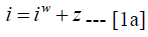
Since the economy is assumed small, rational expectation investors assume that the expected change in exchange rate is the actual rate of change, that is,
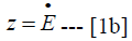
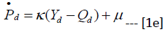
The money sector is described by the LM relation in which interest rate adjusts to changes in money supply. The money sector is at equilibrium when equation (1c) is satisfied
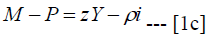
Where ρ measures the rate at which interest rate responds to demand for money.1 Decomposing aggregate general price level to the prices of oil, domestic industrial goods and price of imported goods, equation 1c’ tells us the composition of general price level
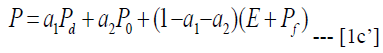
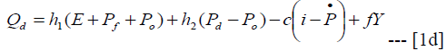
Where Pf is aggregate price of foreign goods. The parameters measure the weight of the price of each sector in aggregate price level. The industrial output is driven by prices of industrial and oil goods, exchange rate, interest rate and the aggregate output. The specification is provided in equation 1(d)
The  is the equilibrium general price level. Recall that industrial prices are assumed sticky, it is
easily predictable. Hence, we can assume that by reverting to the historic behavior of the prices,
it is easy to have a rough guess of what the current price of the industrial goods will be. In this
regard, we assume that the current (equilibrium) price level is the difference between demand
and supply of manufacturing goods and the expected secular rate of inflation, μ.
is the equilibrium general price level. Recall that industrial prices are assumed sticky, it is
easily predictable. Hence, we can assume that by reverting to the historic behavior of the prices,
it is easy to have a rough guess of what the current price of the industrial goods will be. In this
regard, we assume that the current (equilibrium) price level is the difference between demand
and supply of manufacturing goods and the expected secular rate of inflation, μ.
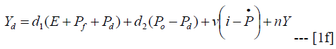
the demand for industrial output is also determined by exchange rate, relative prices of oil and industrial goods, interest rate, actual general price level and aggregate output. The industrial demand specification is presented in equation (1f)
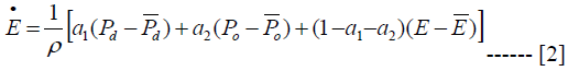
Following the small economy assumption, foreign prices and foreign interest rate are given, so that Pf = if = 0 . Having set up the structure of the economy, we now find the solution values for
the equilibrium flexible price  , the sticky price
  and the exchange rate
  . The solution
values for these three variables are presented in equation 2, equation 3 and equation 4. The
proofs of the equations are provided in appendix.
. The solution
values for these three variables are presented in equation 2, equation 3 and equation 4. The
proofs of the equations are provided in appendix.

Equations 2, 3 and 4 say that the equilibrium price of each of the variables depends on the deviation of own and the other variables from their respective long run value and the parameters that define the structure of the system. The equation system contains three equations in three unknowns and hence, it is a 3x3 equation system which can be expressed in matrix form shown in equation A11 in the appendix. The characteristic polynomial determinant of the system is given as (B-PI) = 0 where B is the 3x3 matrix, P is a column vector of prices and I is identity matrix. The characteristic roots of the solution are bi, b2 and b3. The bs are expected to be negative so as to ensure long run convergence, so that
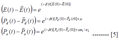
Equation 5 shows the that each variable converges to its long run time path at rate β and for course any possible expected inflation rate captured by μ. Combining equations 2 and 5, we can determine the spot exchange rate and then inspect how monetary shocks will impact on the spot exchange rate. The solution value in this regard is given in equation 6
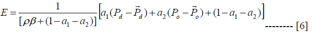
We can also solve for the current price of oil using equation 6. A little manipulation of this equation provides a solution value for the current price of oil as shown in equation 7
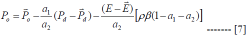
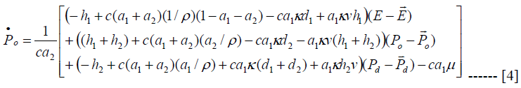
Equation 6 says that the deviation of exchange rate from its long run is a function of the deviation of the prices of industrial goods and oil from their long run and also a function of the response of interest rate to money demand, the price of import goods and finally the long run adjustment coefficient. Oil price and industrial price deviation has direct effect on exchange rate deviation while other variables has inverse effect. The explanation for equation 6 can be implied for equation 7 as well. Now it is time to establish our key equations, that is, equation for overshooting. Consider a monetary expansion. How will current oil price respond? The answer is provided when we differentiate equation 7 with respect to monetary expansion, that is,
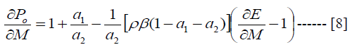
This equation was derived based on the assumption that in the long run, changes in long run
prices and money are the same while industrial price does not respond to monetary shock, that is, 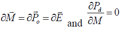 . Equation 8 is one of the two key equations for price overshooting.
The equation says that the response of oil price to monetary shock depends on the response of
exchange rate to monetary shocks, interest rate, the adjustment coefficient and of course the
relative price of oil and industrial good and then, finally the price of imported goods. Equation 8
tells us the situation under which oil price overshooting exists and by what magnitude. Suppose
there is no exchange rate overshooting, that is,
. Equation 8 is one of the two key equations for price overshooting.
The equation says that the response of oil price to monetary shock depends on the response of
exchange rate to monetary shocks, interest rate, the adjustment coefficient and of course the
relative price of oil and industrial good and then, finally the price of imported goods. Equation 8
tells us the situation under which oil price overshooting exists and by what magnitude. Suppose
there is no exchange rate overshooting, that is,  . This means that exchange rate adjusts
instantaneously to monetary shock. This can exist if capitals are perfectly mobile and of course
assets are perfectly substitutes. In this regard, there will not be any presence of the arbitragers.
If this is the situation, equation 8 reduces to
. This means that exchange rate adjusts
instantaneously to monetary shock. This can exist if capitals are perfectly mobile and of course
assets are perfectly substitutes. In this regard, there will not be any presence of the arbitragers.
If this is the situation, equation 8 reduces to  , the value that is greater than 1. The
interpretation of this is that oil price will overshoot largely following monetary expansion if
exchange rate is perfectly flexible. The magnitude of the overshooting depends strictly on the
size of the relative price. The higher the price of industrial good, the larger will the short run oil
price overshoots its long run. Suppose there is no industrial sector, which means a1 = 0 while oil
price adjust instantaneously, indicating that a2 = 1 then of course oil price will not overshoot its
long run. What this suggests is that oil price is flexible to the extent that the change in monetary
expansion has a proportionate change in oil price. The third scenario is when we relax the
assumption of no exchange rate overshooting and of course there is industrial sector. This means
that the impact of monetary shock on oil price will be minimal because exchange rate will absorb
part of the shock, and so, there are both oil price and exchange rate overshooting. Generally, in
the face of imperfect capital mobility and when assets are not perfectly substitute, monetary
shock will cause oil price overshooting and exchange rate overshooting. Which is greater
depends on the extent of flexibility. The more flexible is the price, the less overshooting will the
impact of monetary expansion. Also, oil price overshooting depends on the weight of relative
prices, interest rate, and the speed of adjustment to long run. The larger the size of any of the
parameters, the smaller the amount of overshooting. It must also be noted from equation 8 that if the values of the parameters are large enough and the exchange rate overshoots, then oil price
can undershoot its long run.
, the value that is greater than 1. The
interpretation of this is that oil price will overshoot largely following monetary expansion if
exchange rate is perfectly flexible. The magnitude of the overshooting depends strictly on the
size of the relative price. The higher the price of industrial good, the larger will the short run oil
price overshoots its long run. Suppose there is no industrial sector, which means a1 = 0 while oil
price adjust instantaneously, indicating that a2 = 1 then of course oil price will not overshoot its
long run. What this suggests is that oil price is flexible to the extent that the change in monetary
expansion has a proportionate change in oil price. The third scenario is when we relax the
assumption of no exchange rate overshooting and of course there is industrial sector. This means
that the impact of monetary shock on oil price will be minimal because exchange rate will absorb
part of the shock, and so, there are both oil price and exchange rate overshooting. Generally, in
the face of imperfect capital mobility and when assets are not perfectly substitute, monetary
shock will cause oil price overshooting and exchange rate overshooting. Which is greater
depends on the extent of flexibility. The more flexible is the price, the less overshooting will the
impact of monetary expansion. Also, oil price overshooting depends on the weight of relative
prices, interest rate, and the speed of adjustment to long run. The larger the size of any of the
parameters, the smaller the amount of overshooting. It must also be noted from equation 8 that if the values of the parameters are large enough and the exchange rate overshoots, then oil price
can undershoot its long run.
The second key equation is the effect of monetary shock on current exchange rate. Just like the case of oil price, the magnitude and direction of exchange rate overshooting depends on the nature of the economy and whether oil price have proportionate response to monetary shock or not. The overshooting also depends on the speed of adjustment, interest rate response to money demand, relative price and of course price of imported goods. We also use equation 6 to derive the nature and magnitude of exchange rate overshooting. Still assuming constant prices in the long run, the response of exchange rate to monetary shock is provided in equation 9
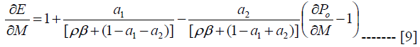
There is a direct impact of prices on exchange rate overshooting. In the absence of oil price
overshooting, exchange rate accounts for the entire effect of monetary shocks, having a high rate
of overshooting. Suppose oil sector is not considered in the model and assume an instantaneous
adjustment of industrial price to shocks. In this case, a2 = 0 and a1 =1, hence, equation 9
reduces to  which is positive. This outcome is the basic Dorbusch overshooting solution
and it says that exchange rate will overshoot its long run when there is monetary shock and the
industrial sector adjusts instantaneously. Also, the equation informs us that the magnitude of the
overshooting depends on the response of interest rate to money demand and the speed of
adjustment to the long run. The higher the interest rate or speed of adjustment, the lower the size
of overshooting.
which is positive. This outcome is the basic Dorbusch overshooting solution
and it says that exchange rate will overshoot its long run when there is monetary shock and the
industrial sector adjusts instantaneously. Also, the equation informs us that the magnitude of the
overshooting depends on the response of interest rate to money demand and the speed of
adjustment to the long run. The higher the interest rate or speed of adjustment, the lower the size
of overshooting.
It is clear from equations 8 and 9 that so long as the oil price and exchange rate do not adjust instantaneously to monetary shock, the two prices will overshoot their long run. Which is stronger depends on the size of relative price. We can use the same idea to solve for industrial price overshooting but since the focus is on these two prices, it is limited to the two key equations.
Technique of Data Analysis
Following equations 2, 3 and 4, all the variables are interdependent and need to be estimated simultaneously. There are basically two ways of estimating economic variables that are interdependent as shown in these equations. The first approach is to develop a dynamic stochastic general equilibrium (DSGE) where the objective functions and constraints are explicitly specified. The advantage of employing this statistical method is that the parameters of the DSGE are very useful for policy prescription in the sense that it possesses the ability to clearly answer policy-related issues and makes prescriptions easily understood.
Alternatively, a panel autoregressive (Panel VAR) can be employed. The panel VAR technique eschews some of the complex restriction placed on the parameters of the DSGE2. The VAR model has the capacity to capture the dynamic interdependence present in equations 8 and 9. To estimate Panel VAR, three steps must be taken. First an appropriate panel VAR must be specified. Second, a Granger causality test based on the properties of the series is carried out and third, the computation of impulse response function and variance decomposition.
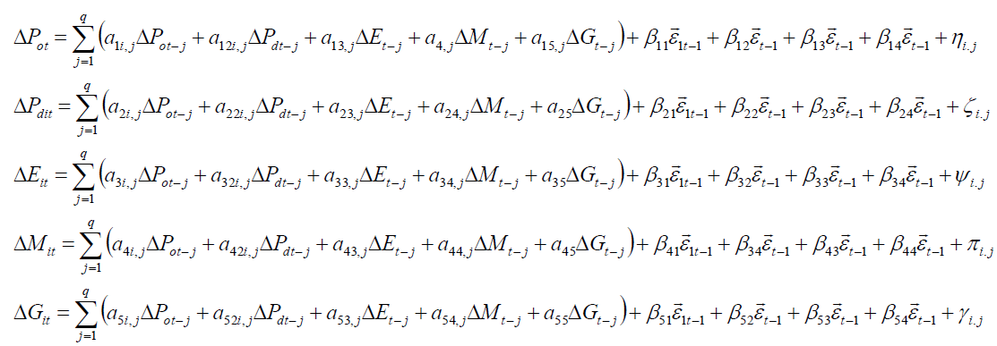
Equation 10 is a panel ECM version of panel VAR, where i represents countries t is time and q is the number of lags that enters the equation, G is the log GDP and are
country-specific fixed effects. Before embarking on the use of VAR, two other considerations
must be observed. First, the level at which the variables are stationary. This condition is
important because the Granger causality test, which is the key test for VAR relies on the fact that
the series should be stationary. The Second is to find out if the series cointegrates or not. The
coingegration condition is to ensure long run convergence. Based on the nature of the series, all
the variables are stationary at first difference and the maximum lag is 1. Thus, the method is a 5-
variable panel VAR of order 1, that is PVAR (1) or panel VECM (P-VECM). The second step is
to carry out Granger causality test. The Granger causality test is prominent in panel data
analysis. By definition, Granger causality tests, as it is relevant to this study, shows whether
each of the variables can predict others and if the lagged values of the variables can provide
information about each endogenous variable.
are
country-specific fixed effects. Before embarking on the use of VAR, two other considerations
must be observed. First, the level at which the variables are stationary. This condition is
important because the Granger causality test, which is the key test for VAR relies on the fact that
the series should be stationary. The Second is to find out if the series cointegrates or not. The
coingegration condition is to ensure long run convergence. Based on the nature of the series, all
the variables are stationary at first difference and the maximum lag is 1. Thus, the method is a 5-
variable panel VAR of order 1, that is PVAR (1) or panel VECM (P-VECM). The second step is
to carry out Granger causality test. The Granger causality test is prominent in panel data
analysis. By definition, Granger causality tests, as it is relevant to this study, shows whether
each of the variables can predict others and if the lagged values of the variables can provide
information about each endogenous variable.
Alongside the P-VECM is the computation of the impulse response and variance decomposition. The impulse response functions (IRFs) show the effects of shocks on the adjustment path of the variables in the panel VECM model. Impulse Response Functions can also be graphically presented showing the effect of shocks on the current and future path of the variables under consideration. Variance decompositions measure the contribution of each type of shock to the forecast error variance.
Variable Measurement and Sources of Data
From equations 10, the variables for which data are to be obtained are oil price, industrial price, exchange rate, money supply and GDP. This study utilizes data on these variables for 20 major oil producing nations comprising 10 OPEC and 10 non-OPEC members from 1991 to 20153. The countries are selected based on their relevance to the world oil production and consumption and population. Data on money supply (M), oil price (oil), industrial price (indi) are obtained from the International Financial Statistics (IFS) published by the World Bank Group. Real effective exchange rates (exch) are extracted from the Bank of International Settlement while the gross domestic products (GDP) are obtained from the World Development Indicators (WDI). International oil prices (brent) are measured in US dollar per barrel ($/pb). The proxy for industrial prices is the producer price commodity index.
Results and Discussion
The descriptive statistics of all the variables is presented in Table 4.1. On average oil price and industrial prices between 1991 and 2015 posted $38.84 and 59.74 respectively. The average real effective exchange rate was 108.7. Further, GDP and money supply averaged $124.22 billion and $116.28 billion respectively in Table 1.
| Table 1 Descriptive Statistics of the Variables | |||||
| Variables/Statistics | GDP | oil | M | exch | indi |
| Mean | 124.22 | 38.84 | 116.28 | 108.67 | 59.74 |
| Maximum | 865.97 | 133.88 | 454.88 | 546.04 | 751.61 |
| Minimum | 20.05 | 11.34 | 1.00 | 34.53 | 4.18 |
| Std. Dev. | 265.92 | 28.43 | 511.00 | 54.24 | 50.93 |
| Skewness | 3.87 | 1.14 | 6.16 | 3.76 | 3.76 |
| Kurtosis | 18.29 | 2.97 | 43.46 | 21.85 | 50.58 |
| Jarque-Bera | 856.88 | 150.93 | 521.72 | 12027.19 | 67697.14 |
| Probability (Jarque-Bera) | 0.000 | 0.000 | 0.000 | 0.000 | 0.000 |
| Observations | 500 | 500 | 500 | 500 | 500 |
Maximum obtainable values for GDP, oil price, money supply, effective exchange rate and industrial prices within the sample period of 1991 to 2015 are 865.97, 133.88, 454.88, 546.04 and 751.61 respectively. The minimum obtainable value of each variable is 20.05, 11.34, 1.00, 34.53 and 4.18 respectively. The relative stability and volatility in the variables are indicated by the standard deviation statistics. The rule of thumb is that a value closer to 0 is stable and less volatile while a value farther from 0 is less stable and more volatile. Table 4.1 indicates that all the variables are highly volatile with money supply being the most volatile and oil price being least volatile. GDP is the third least volatile while exchange rate follow suit. This gives first hand information about the presence of overshooting and the facts that oil price indicate relatively faster adjustment than exchange rate and industrial price.
The skewness statistics which is an indicator of normality distribution of the series shows that all the variables are positively skewed while the kurtosis statistics shows only oil prices is lowly peaked. The Jarque – Bera statistic shed more light to the normality properties of the series. As can be observed, all the series are not normally distributed (see the probability of Jarque-Bera), suggesting that firs, ordinary least square method cannot be appropriate for estimating equation 10 and second, further tests are required to ascertain the appropriate technique of estimation. Unit root tests that shows the nature and level of the absence of unit root or the presence of statinarity and cointegration tests that is required for long run relationship are performed and the results are presented in Tables 2 & 3 respectively.
| Table 2 LEVIN, LIN, CHU Unit Root Test | ||||||||||
| VARIABLE | LEVEL | FIRST DIFFERENCE | ||||||||
| 1 | 2 | 3 | 1 | 2 | 3 | I(d) | ||||
| Money supply | 1.068 | 0.119 | 8.779 | 2.463 | -0.550* | 0.452 | I(1) | |||
| Effective exchange rate | 2.925 | 0.923 | 1.515 | -1.227 | -5.899* | -12.762* | I(1) | |||
| GDP | 2.904 | 1.945 | 1.739 | -4.696 | -7.830* | -3.250* | I(1) | |||
| Oil prices | 1.010 | 5.457 | -1.411 | -2.965 | 1.228 | -18.123* | I(1) | |||
| Industrial prices | 1.187 | 0.832 | 6.043 | -1.796 | -3.874* | -4.039* | I(1) | |||
| Im, Pesaran, Shin unit root test | ||||||||||
| VARIABLE | LEVEL | FIRST DIFFERENCES | ||||||||
| 1 | 2 | 1 | 2 | I(d) | ||||||
| Money supply | 1.390 | 1.388 | 1.647 | -1.901 | I(1) | |||||
| Effective exchange rate | 3.752 | 0.957 | -9.519* | -7.936* | I(1) | |||||
| GDP | 1.707 | 1.268 | -6.510* | -6.918* | I(1) | |||||
| Oil prices | 1.613 | 0.922 | -12.312 | -8.907* | I(1) | |||||
| Industrial prices | 2.030 | 1.858 | -4.544* | -4.752* | I(1) | |||||
| Table 3 Result of Johansen’s CO Integration Test | ||||
| Hypothesized No. of CE(s) |
Fisher Stat.* (from trace test) |
Prob. | Fisher Stat.* (from max-eigen test) |
Prob. |
| None | 374.9 | 0.0000 | 244.4 | 0.0000 |
| At most 1 | 209.8 | 0.0000 | 357.3 | 0.0000 |
| At most 2 | 102.7 | 0.0000 | 70.68 | 0.0002 |
| At most 3 | 52.57 | 0.0219 | 42.07 | 0.1612 |
| At most 4 | 34.78 | 0.4309 | 34.78 | 0.4309 |
Both Levin, Lin, Chu and Im, Pesaran, Shin panel unit root presented in Table 2, indicates that all the series have unit root at level but no evidence of unit root at first difference. This implies that all the series are stationary at first difference.
Following the level of stationarity of the series, a long run cointegration test is performed and the result is presented in Table 3. The results is used to discuss the long-run effects of money supply on oil prices, industrial prices, exchange rates and gross domestic income for the oil producing countries in the world.
The error correction equation from none to at most 3 show that the variables are none cointegrated while the error correction equation of at most 4 show that all the variables are cointegrated using Fisher trace test. Using Fisher max-eigen test, the error correction equation from none to at most 2 show that the variables are none cointegrated while the error correction equation of at most 3 and 4 show that the all the variables are cointegrated therefore we accept the null hypothesis that the variables are co integrated. Thus we have four cointegrating equation in the model and equation 10 reflects this information.
Since all the series are integrated of order 1, then panel vector error correction (PVECM) is estimated. It must be recalled that a crucial prerequisite for the use of the panel VECM is that all variables in the model must be non-stationary (stationary) at first difference. The tests in tables 4.2 and 4.3 satisfy this condition and so, the result of the PVECM is presented in Table 4.4.
Table 4 reports the results of the panel vector error correction arising from equation 10. The outcome of the cointegrating test in Table 3 suggests 4 cointegrating equation in the 5x5 equation system. Thus, the error corrections are given as EC1, EC2, EC3 and EC4. Each of these error corrections tells us the speed of adjustment to long run equilibrium. The ECi (I = 1,2,3,4) are the coefficients βs in equation 10. The results show that the error-correction term for oil prices (EC1) is negative (-0.016) and significant while the error correction of industrial prices is positive (0.0006) and insignificant. This implies that in the oil producing nations, there is evidence of oil price and industrial price overshooting in the short run following money supply shocks. However the adjustment to long run equilibrium differs. While oil price falls gradually to adjust to its long run equilibrium, industrial prices fails to adjust. In particular, the oil prices equation suggest that a short-run overshooting from the long-run money supply relationship requires oil to fall gradually to correct long-run disequilibria with the short-run overshooting.
| Table 4 Results of Panel Vector Error Correction Model | |||||
| Δ(Oil prices)t | Δ(Industrial prices)t |
Δ(Exchange Rates)t |
Δ(GDP)t | Δ(Money supply)t | |
| EC1 | -0.016** [-2.767] |
-0.0015 [-0.311] |
2.341*** [ 5.625] |
-0.501 [-0.966] |
0..7701*** [ 8.784] |
| EC2 | 0.006** [ 2.767] |
0.0006 [ 0.311] |
-0.963*** [-5.625] |
0.845 [ 0.966] |
-0..4113*** [-8.784] |
| EC3 | 0.0001** [ 2.767] |
0.00001 [ 0.31167] |
-0.015*** [-5.625] |
0.554 [ 0.966] |
-0.150*** [-8.784] |
| EC4 | 0.0000000001** [ 2.767] |
0.000000000001 [ 0.311] |
-0.00000000006*** [-5.625] |
0.00005 [ 0.966] |
-0.290*** [-8.784] |
| Δ(Oil prices)t-1 | -0.411 [-1.269] |
-0.006 [-0.930] |
-0.000000000002 [-0.549] |
-0.0000000003*** [ 10.225] |
|
| Δ(Industrial prices)t-1 |
-2.430** [-2.366] |
0.015 [ 0.932] |
0.0000000002 [ 0.548] |
-0.0000000001*** [-10.273] |
|
| Δ(Exchange Rates)t-1 |
-1.441* [-1.751] |
2.712 [ 0.941] |
-0.000000004 [ 0.548] |
0.00000000001*** [-11.338] |
|
| Δ(GDP)t-1 | -0.335* [-1.748] |
0.137 [ 0.937] |
0.219 [ 0.929] |
-0.204*** [-10.208] |
|
| Δ(Money supply)t-1 | 0.163* [ 1.749] |
-0.599 [-0.942] |
-1.0744 [-1.031] |
-4.884 [-0.548] |
|
Further, effective exchange rate and GDP also significantly overshoot their long run equilibria owing to money supply shock. This suggests that when deviating from equilibrium conditions due to money supply shocks, exchange rate and GDP also adjusts to correct long-run disequilibria. Using their error correction term in the exchange rate model, EC3 = -0.015 suggesting that a short-run overshooting from the long-run money supply relationship requires exchange rate to fall (appreciate) to restore the long run equilibrium, while the error correction term in the GDP model, EC4=0.00005, implies that GDP must rise to correct long-run disequilibria with the short-run overshooting in selected oil producing nations. The GDP sluggishly adjusts to long run compared to other variables.
Further, the absolute values of the two error-correction terms indicate that, with money supply shocks, oil prices seem to adjust more quickly than industrial (sticky) prices to achieve the long run equilibrium, thereby affecting relative prices in the short-run. This result is in line with the work of Baek and Miljovik (2018). The second error-correction term (EC2) in the short run oil prices model is positive (0.006) and significant, meaning that in the short run, oil prices must increase when industrial prices overshoot their long-run equilibrium. This result is consistent with equation 4 where it is proposed that deviation of industrial price from its long run (overshooting) will cause current oil price to increase. Monetary expansion could lead to increase in money demand, thereby increasing demand for industrial goods, causing increase in industrial price. The increase in demand also causes more demand for oil in production, leading to increase in oil price. In the same vein, exchange rate overshooting and GDP overshooting all have positive effect on oil price (0.0001 and 0.0000000001 respectively). This is not implausible because depreciation of exchange rate due to expansionary money supply will also ease production which invariably leads to demand for more oil for production and hence increase in oil price. A cursory look at the magnitude suggests that there is a mild effect on the short run oil price of the exchange rate and GDP overshooting. This outcome supports the solution value in equation 4.
The first error-correction term (EC1) in the industrial prices model is negative but not significant (-0.0015), indicating that oil price overshooting does not significantly affect industrial price in the short run. However, the error-correction (EC1) positively and significantly affect exchange rate. It is also observed that the error-correction term (EC2) in exchange rate model is negative and significant but positive and insignificant in the GDP model. Also, the error-correction term of exchange rate (EC3) show positive but insignificant effect on industrial price and GDP but show negative and significant effect on exchange rate model.
Next is how the short run oil price, industrial prices, exchange rate and GDP respond to the lag of the variables. Increase in lagged industrial price leads to increase in oil price (Table 4). Also, increase in the previous exchange rate has negative impact on oil price. In particular, a 1% increase in industrial price and exchange rate will lead to 2.4% and 1.44% decrease in oil price respectively. Further, a 1% increase in the last period GDP and money supply will engender oil price increase to the tune of 0.34% and 0.15% respectively. Hence, industrial price has the greatest impact on oil price in the short surn, followed by money supply, then exchange rate and lastly GDP.
Next is the causality result, showing which of the variables causes which. A cursory look at the result reveals that there are more of unidirectional causality than feed back or no causality (Table 5). For instance, GDP and money supply Granger cause oil price while money supply Granger causes GDP. This suggests that monetary shock has both direct and indirect causation on oil price. The direct causation is the one running from monetary shock to oil price and the indirect causation is the one that runs through GDP. It is also revealed that oil price shock causes industrial price and effective exchange rate while industrial price causes effective exchange rate. Therefore, exchange rate overshooting is caused by oil price directly and indirectly through industrial price. There is no other causation noticed in the Table.
| Table 5 VEC Granger Causality/Block Exogeneity Wald Tests | |||||||||||||||
| Dep. Variable D(Oil Prices) |
Dep. Var D(Ind Prices) |
Dep. Variable D(REER) |
Dep. Variable D(GDP) |
Dep. Variable D(M2) |
|||||||||||
| Excluded | chi-sq | df | prob | chi-sq | df | prob | chi-sq | df | Prob | chi-sq | df | Prob | chi-sq | df | prob |
| D(OIL_PRICE) | 12.32 | 2 | 0.002* | 30.84 | 2 | 0.000* | 1.1 | 2 | 0.62 | 2.17 | 2 | 0.337 | |||
| D(IND_PRICES) | 1.032 | 2 | 0.596 | 8.551 | 2 | 0.013* | 0.6 | 2 | 0.73 | 0.46 | 2 | 0.796 | |||
| D(REER) | 0.496 | 2 | 0.78 | 4,771 | 2 | 0.092 | 4.7 | 2 | 0.06* | 0.6 | 2 | 0.742 | |||
| D(GDP) | 6.377 | 2 | 0.041* | 0.119 | 2 | 0.942 | 0.007 | 2 | 0.996 | 0.01 | 2 | 0.994 | |||
| D(M2) | 15.07 | 2 | 0.0005* | 0.075 | 2 | 0.962 | 1.842 | 2 | 0.398 | 13 | 2 | 0.002* | |||
Impulse Response Functions and Variance Decomposition
Impulse response function provides specific information about the impacts of shocks on the adjustment path of the variables in the panel VECM model. Figure 4.1 reports that a shock of industrial prices have a negative impact to the oil price from the fourth year to the tenth year. It also reports that oil price shock has a negative impact to the industrial prices from the eight year to the tenth year. It is also revealed that money supply responses to oil prices and industrial price to be positive and negative respectively. Exchange rate responds to oil prices and industrial price positively and negative respectively while GDP response to oil prices and industrial price is positive and negative respectively.
We now turn to the outcome of the variance decomposition. Variance decomposition tells us how much of a change in a variable is due to its own shock and how much due to shocks to other variables. In the short run, most of the variations is due to own shock. But as the lagged variables’ effect starts manifesting, the percentage of the effect of other shocks increases over time. Both Impulse Response Functions and Variance Decomposition computations are useful in assessing how shocks to economic variables reverberate through a system.
The variance decomposition results reported in Table 6 shows that within the periods considered, 97.555% of innovations of the global oil prices are explained by industrial prices past values, yet only 2.221% is explained by its own past values, and exchange rate, gross domestic product and money supply past values contributes less than one percentage. While 98.3% of innovations in the industrial values are explained by its own past values, and 1.401% is explained by oil prices past values, and exchange rate, gross domestic product and money supply past values contributes less than one percentage. Innovation of the exchange rate is attributed to 98.29 and 1.492 of industrial prices and oil prices past values and less than one percentage in its own past values, gross domestic product and money supply past values and this is also the same for gross domestic product, where the innovations is largely dominated by industrial prices followed by oil prices while exchange rate, gross domestic product and money
| Table 6 Variance Decomposition Result: (Full Sample) | |||||||
| Variance Decomposition of oil prices | |||||||
| Period | S.E. | OIL_PRICE | IND_PRICES | REER | GDP | M2 | |
| 1 | 17.306 | 100.000 | 0.000 | 0.000 | 0.000 | 0.000 | |
| 5 | 40.418 | 61.824 | 36.956 | 0.1049 | 0.2033 | 0.910 | |
| 10 | 803.776 | 2.221 | 97.555 | 0.113 | 0.003 | 0.105 | |
| Variance Decomposition of industrial prices | |||||||
| Period | S.E. | OIL_PRICE | IND_PRICES | REER | GDP | M2 | |
| 1 | 14.386 | 0.540 | 99.459 | 0.000 | 0.000 | 0.00 | |
| 5 | 486.561 | 1.347 | 98.477 | 0.101 | 0.00001 | 0.072 | |
| 10 | 15051.177 | 1.401 | 98.385 | 0.114 | 0.00004 | 0.098 | |
| Variance Decomposition of exchange rate | |||||||
| Period | S.E. | OIL_PRICE | IND_PRICES | REER | GDP | M2 | |
| 1 | 1183.057 | 0,120 | 0.652 | 99.227 | 0.000 | 0.000 | |
| 5 | 4480.006 | 1.530 | 60.298 | 37.611 | 0.008 | 0.552 | |
| 10 | 1200001.5 | 1.492 | 98.290 | 0.104 | 0.00003 | 0.112 | |
| Variance Decomposition of gross domestic product | |||||||
| Period | S.E. | OIL_PRICE | IND_PRICES | REER | GDP | M2 | |
| 1 | 56921971680.060 | 0.165 | 0.885 | 0.042 | 98.906 | 0.000 | |
| 5 | 432171909756.706 | 0.132 | 32.601 | 0.071 | 67.119 | 0.075 | |
| 10 | 10095068764066.84 | 1.241 | 97.947 | 0.116 | 0.594 | 0.099 | |
| Variance Decomposition of money supply | |||||||
| Period | S.E. | OIL_PRICE | IND_PRICES | REER | GDP | M2 | |
| 1 | 31406322795684.57 | 2.689 | 0.381 | 0.035 | 0.003 | 96.890 | |
| 5 | 147894702425452.4 | 5.392 | 3.744 | 0.185 | 0.0007 | 90.676 | |
| 10 | 1432230483870907 | 2.882 | 91.281 | 0.240 | 0.0007 | 5.594 | |
Supply values are less than one percentage. While for money supply innovations is still dominated by the industrial prices by 91.28% and 5.59% of its own price and 2.88 of oil prices and exchange rate is less than one percentage. From the interpretation of the variance decomposition results, it can be said that the innovations in industrial prices dominates the multivariate model in the oil producing nations in Figure 1.

Figure 1 Impulse Responses of the Variables: Selected Oil Producing Nations
Conclusion and Policy Implications
Empirical evidence on the relationship among oil price overshooting, industrial price overshooting, monetary policy and economic growth is unambiguously scanty, particularly in the oil producing nations. This study therefore contributes to the empirical literature in this regard. The 20 countries selected covers both OPEC and non-OPEC countries. Annual data for the period 1991-2016 were obtained and panel vector error correction mechanism (P-VECM) in the context of modified Dornbusch overshooting model was estimated. The overshooting results are explained using the error-correction terms of the variables.
The result suggests that oil price, industrial prices and exchange rate overshoot their long run prices. In the case of oil price overshooting, the error-correction model reveals that when oil price overshoots, it has to reduce in order to correct for short run disequilibrium. This result is in line with the work of Saghaian et al (2002), Ratii & Vepignan (2015); Baek & Miljovic (2018) in the case of commodity price. However, in contrast to Baek & Miljovic (2018) and Saghaian et al (2002), the error-correction model for industrial prices indicates that no adjustment is significantly observed. This could be as a result of the nature of the economies under study. Exchange rate also overshoots its long run and the adjustment time path is negative, indicating that exchange rate has to appreciate to compensate for any loss in financial assets informed by expansionary monetary policy. This result is also in line with some empirical works reviewed in this paper. However, in contrast to previous evidence, the speed of adjustment in our result is significant and relatively faster (-0.015). For instance, the speed of adjustment in Saghaian et al. (2002) was 0.0140 (not significant) while that of Baek & Miljovic (2018) was 0.040 (not significant). Meanwhile, our result is in line with the basic Dornbusch (1978) overshooting model. Hence, we conclude that in the oil producing countries, exchange rate significantly overshoots its long run but has to reduce (appreciate) in order to adjust for the short run disequilibrium when there is expansionary monetary expansion.
Other adjustments noticed are that when industrial price or exchange rate or GDP overshoots its long run, oil price will rise. In the same vein, oil price overshooting causes exchange rate depreciation but when industrial price overshoots, exchange rate appreciates. It is also discovered that increase in lagged values of industrial price, and exchange rate cause oil price to fall. But increase in the lagged value of GDP and money supply triggers oil price.
Following these conclusions, some policy implications and recommendations can be drawn. First, monetary shocks in the major oil producing nations will cause oil price to overshoot its long run equilibrium, that is, monetary shocks will cause short run volatility of the oil price. Not only will there be oil price overshooting following monetary shock, industrial price and effective exchange rate will also overreact in the short run. Consequently, when the authorities in these countries wish to increase economic activity (GDP) through monetary expansion, they should anticipate the oil price effect. This is true because the causality result indicates that increase in GDP causes oil price, consequently, monetary expansion leads price overshooting which then triggers industrial price, thereby leading to depreciation. Since it takes a long period for effective exchange rate to recover, it turns out that in oil producing nations, monetary expansion contributes to effective exchange rate depreciation, even after causing overshooting
Further, oil price is more unstable than the industrial prices in these countries particularly when there is money supply shock and consequently, the financial viability of oil investors will be affected tremendously. This instability could cause investors of oil prices sector to reduce their investment in this sector or causes potential investors to become reluctant to invest in these countries.
Oil investors can reduce risk by using techniques such as purchasing oil insurance from the government or private companies, and diversifying their investment to other sector of the economy since there is instability of prices and income both in the short and the long run of the economy. Therefore the investors are advised to diversify their investment in other sector that their incomes are more stable than the energy sector overtime. However, these oil market techniques cannot reduce price and income risks completely but only partially.
Considering the fact that oil prices exhibit more dramatic response to monetary policy instrument than industrial prices, it is advisable to be conscious of the use of monetary policy as its changes could cause make macroeconomic policy be counterproductive. One way of stemming the oil price overshooting is that the majority of oil producing nations should reduce reliance on oil as the sole exporting product and diversify their exporting base since their prices (oil) is more unstable than the exchange rate. This recommendation is even more important in this era where oil is becoming less valuable product overtime. For example oil was more important in the year of 2009 than the year of 2019.
End Notes
1As we shall see later, the parameter shows the rate at which interest rate responds to monetary shocks.
2A multivariate simultaneous equation models can also be employed provided the source of endogeneity is known (Sim, 1980).
3These countries are Algeria, Angola, Brazil, Canada, China, Columbia, Ecuador, India, Indonesia, Iran, Iraq, Kuwait ,Mexico, Nigeria, Qatar, Russia, Saudi Arabia, UK, USA and Venezuela.
References
- Allegreta, J., & M. TaharBenkhodja (2015). External shocks and monetary policy in an oil exporting economy (Algeria). Journal of Policy Modeling. Vol. 37, No. 4:652–667.
- Arezki, R., Z. Jakab, D. Laxton, A. Matsumoto, A. Nurbekyan, H. Wang & J. Yao (2017). Oil prices and the Global Economy. IMF Working Paper No. WP/17/15. Washington D.C, United States of America.
- Baek J, & D. Miljkovic (2018). Monetary policy and overshooting of oil prices in an open economy. The Quarterly Review of Economics and Finance, Vol. 22, 222-245
- Caraiani, P & A. Calin (2019). Monetary policy of energy sector bubbles. Energies. Vol. 2. No. 1:1-13.
- Dornbusch, R ( 1978). Expectations and exchange rate dynamics. Journal of Political Economy, Vol.84, No. 6: 1161–76
- Frankel, J (1986). Expectations and Commodity Price Dynamics. The overshooting model. American Journal of Agricultural Economics. Vol 68, Issue 2: 344-348.
- Gaidar, Y (2007). The Soviet collapse: grain and oil. American Enterprise Institute of Public Research. Available at www.nei.org .
- S. Hammoudeh, J. Hyun & R. Gupta (2017). Oil price shocks and China's economy: Reactions of the monetary policy to oil price shocks. Energy Economics. Vol.62, Issue C: 61–69.
- Leduc, S & K. Sill (2004). A quantitative analysis of oil-price shocks, systematic monetary policy, and economic downturns. Journal of Monetary Economics. Vol.51, issue 1:781–808
- Miljkovic, D. & J. Baek (2019). Monetary impacts and overshooting of energy prices: the case of the U.S. coal prices. Minerals Economics, Vol. 32, No. 3:317-322.
- Olubiyi, & P. Olapade (2018). On the efficiency of stock market: a case of selected OPEC member country. Central Bank of Nigeria Journal of Applied Statistics, Vol. 9, No. 2:75-101.
- Olubiyi, E (2019). Are stock prices behaviors of OPEC countries interdependent? Nigerian Journal of Securities Market Vol. 4, No. 1:1-27
- Plantep, M (2014). How should monetary policy respond to changes in the relative price of oil? Journal of Economic Dynamics & Control, 44:1-19.
- Rahman, S., & A. Serletis (2010). The asymmetric effects of oil price and monetary policy shocks: a nonlinear VAR approach. Energy Economics 32, 6: 1460–1466.
- Ratti, R & J. Vespignani (2015). Oil prices and global factor macroeconomic variables. Energy Economics. Vol. 59:198-212.
- Razmi, F., M. Azali, L. Chin & M. Habibullah (2016). The role of monetary transmission channels in transmitting oil price shocks to prices in ASEAN-4 countries during pre- and post-global financial crisis. Energy Vol.101, 581-591.
- Robertson, J., & D. Orden (1990). Monetary impacts on prices in the short and long run: some evidence from New Zealand. American Journal of Agricultural Economics. 72 (1):60–71.
- Saghaian, S., M. Reed, & A. Marchant, M (2002). Monetary impacts and overshooting of agricultural prices in an open economy. American Journal of Agricultural Economics. 84 (1): 90-103.
- Smith, G., A. Rascouet & W. Mahdi (2015). OPEC won’t cut production to stop oil’s slump. Business – Blumberg. Available at https://www.bloomberg.com/news/articles/2015-12-04/opec-maintains-crude-production-as-group-defers-output-target-ihryzilb.