Keywords

Compensation Discrimination, Sports Economics, US Major League Baseball.

Introduction

Racial discrimination in sports has been an on-going subject of study for more than four decades. Professional sports were largely segregated by race for many years. Initially, the primary venues open to non-white professional athletes in the US were segregated non-white teams. In terms of professional baseball, racial integration of previously all white teams began with the ground breaking entry of Jackie Robinson in 1947. Since that time, we have seen professional sports become a melting pot of races and nationalities but there has been continuing concern that white and non-white players may not be treated equally.

Scully, 1973, suggests that racial discrimination in US professional sports was far from gone even after some 30 years since the integration of professional baseball. Studies of racial discrimination have mainly focused on pay disparities, but there are other forms of discrimination besides pay that could come into play. Examples of non-salary related discrimination include Conlin & Emerson 2006, who found that non-white players actually have a higher probability of having an active contract and start more games in the US National Football League (NFL) than whites. On the other side of the coin, Madden 2004, finds that non-white coaches in that same league are held to significantly higher standards for hiring and retention than are white coaches.

Work regarding pay discrimination has returned contradictory results as well. For instance, Keefer (2013), Berri and Simmons (2009) and Gius, M. & Johnson, D. (2000) find evidence of racial pay discrimination in the NFL, while Ducking, Groothuis & Hill (2014) find no evidence of pay discrimination by race in the same sport. The authors (2015 and 2013), using more recent data from the NFL also find that there is no significant racial pay discrimination at least among rookie salaries, suggesting that overt discrimination in pay may no longer be de rigueur.

Evidence regarding pay discrimination from other sports is also somewhat mixed. As an example, Jones & Walsh (1988) find evidence that French Canadian defensemen suffered pay discrimination in the National Hockey League while Kahn, 2000, indicates that there is little to no pay disparity in the National Basketball Association. Generally, as newer techniques such as rank-based groupings like the Oaxaca-Blinder decomposition and quintile regression techniques are applied to existing data, researchers have been able to parse out differences across groups more readily that previous methods but have still been unable to come to any unified conclusions about pay discrimination across professional sports.

We extend the line of inquiry into racial differences in professional sports to Major League Baseball (MLB) in the US and widen the analysis to include both pay discrimination and differences in playing time. We find that among the most talented segment of players there is a significant difference in pay and playing time with non-white players being paid more and played more, over and above any differences that would be attributable to measured skill characteristics. This may result from fan preferences if the fan base considers something beyond win/loss record or play-off wins (could there be a feeling that certain teams will be perennial division winners, so that the home team need merely do relatively well to deserve fan loyalty?). If fans prefer non-white players over white players, the choice to discriminate against white players may be profit maximizing even if that choice does not appear to be an optimal policy to maximize winning records.

Data

We create an original data set comprised exclusively of outfielders from the 2015 season of US Major League Baseball. Outfielders, rather than pitchers, are used because there are more outfielders and there is a nearly even split between white players and those identified as non-white as well as the rather large number of skill characteristics available for outfielders. Player statistics include annual salary, number of games played during the season, race and a host of measurable skill based outcomes. Skill characteristics for outfielders include ‘at bats’, runs, hits, double plays, triple plays and home runs. From that raw data, we calculate ‘Slugging’ as a composite skill characteristic. Slugging or Slugging Percentage, is a measure of hitting talent, first suggested by Chadwick, 1867, as average bases per game (later altered to average bases per at bat and accepted in that form by the National League as an official statistic in 1923 and American League in 1946). It is a weighted average of base hits, double plays, triple plays and home runs, divided by at bats, to provide an average number of bases per at bat (with walks specifically omitted as they are not considered as and at bat). Specifically, it weights the hits by the number of bases obtained in each play so that base hits (B) are multiplied by 1 since those hits achieve a single base, while double plays (2B) are multiplied by 2 as they achieve 2 bases, with triple plays (3B) multiplied by 3 and home runs (HR) being multiplied by 4. This weighted number of hits is then divided by at bats (AB) so that Slugging, SLG, is an average number of bases achieved per at bat. Equation 1 summarizes this statistic.

Summary statistics are shown in Table 1 for the overall group and by race. The data set consists of all 208 outfielders that played in 2015, with 108 of those being white and the remainder identified as non-white. Player race was determined by the creation of a panel of reviewers who looked at published baseball cards for each player and determined whether an individual player was ‘white’ or ‘non-white’. The panel consisted of 3 individuals, to avoid the instances of a tie. There were very few cases of a split vote from the panel. At first blush, a comparison across sub-groups shows a significant difference only in salary, with non-whites receiving higher salary at 10% significance.

Table 1 Data Summary 2015 US Baseball Outfielders by Race+
Variable	Overall	Non-Whites	Whites	Difference#
Salary	$3,224,800 ($5,148,055)	$3,901,791 ($5,403,394)	$2,591,689 ($4,836,841)	$1,310,102* Test=1.837056 Ƿ=0.033846537
GamesPlayed	527.4856 (510.7561)	583.45 (571.5714)	475.6852 (443.594)	107.7648 Test=1.510649 Ƿ=0.066287495
SLG	0.3991827 (0.0960257)	0.39519 (0.0924619)	0.4028796 (0.0994983)	-0.00769 Test=-0.5773 Ƿ=0.28204089
White	0.5167
n	208	100	108
Sources: Player data from Baseball Reference at www.baseball-reference.com/players/ Salary data from: Sportrac www.spotrac.com/mlb/rankings/outfield/ +Standard deviation in parentheses Test=test statistic Ƿ=p-value #Difference=Non-White less White *Significant at 10%. **Significant at 5%. ***Significant at 1%.

Models

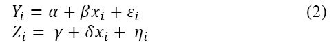
Initially, we begin with a traditional OLS regression with a binary racial identifier and slugging as a composite skill variable for both the natural log of salary (LnSalary) and games played (Games Played). We continue by running a system of seemingly unrelated regressions using the natural log of salary and games played as dependent variables with a binary racial identifier and the composite skill variable as independent variables. The process of seemingly unrelated regression, following Zellner, 1962, provides a joint regression where the equations are likely to have related error terms even though they have different dependent variables. In this case the functions for player i’s earnings Y_i and number of games played, Z_i, are run against a matrix of independent variables, x_i including a racial identifier. Equation 2 shows the system.

These traditional approaches, either OLS or seemingly unrelated regressions, estimates parameters at the conditional mean for each independent variable and are highly efficient but are quite sensitive to outlier values. An additional drawback to traditional estimation techniques is that they assume a normal distribution for the error terms. The case at hand, athlete salaries and games played, is one that is particularly prone to outliers and may be subject to non-normality if different segments of players are treated in different ways.

To take into account the issues of outliers and possibilities of non-normal distributions, we follow Keefer (2013) and others, in expanding the analysis to the use of quintile regressions (Koenker & Bassett, 1978), which is far more robust to the presence of outliers and separates out

groups that may be treated differently (top versus middle versus lower level players). Quintile regressions separate the data into groups ranked by the value of the dependent variable. This allows for the effect of the independent variables to vary, meaning that highest paid players may be treated differently from players at the middle or lower level of salary or that the players that have the highest number of games played may differ from players who played closer to the average number of games or the fewest games. The assumption is that the each θ^th segment of the dependent variable is a linear combination of the independent variables, so that each group is run on the same independent variables but with separately estimated parameters. There are several examples of quintile regression in the sports labour market literature, including Keefer (2013), the authors (2013 and 2015) and Vincent and Eastman (2009), among others.

We use sub-groups of the lowest 25%, median or central group and upper 25% (listed as 25%, 50% and 75%), so that there are 3 divisions (θ=3). Regression results are then obtained for each of the sub-groups. Essentially, the linear relationship between the independent variables, including a race binary variable, for either salary or number of games played is estimated in each of the three groups. Evidence about discrimination is found from tests on the estimated coefficient on the binary racial identifier variable within each group.

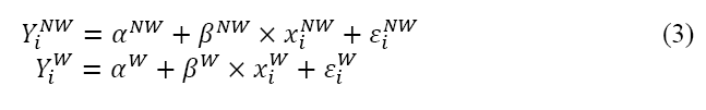
Another technique we use involves breaking the data into two groups by race, then estimating each group before comparing the results. This process is known as the Oaxaca-Blinder decomposition. In general, using NW as the designator for the non-white group and W for the white group. The model is estimated for the set of independent variables (x_i,) for each of the independent variable (Y). This specification allows the difference between estimators by race to be used for hypothesis testing and inference (Melly 2006 and Keefer 2013). Equation 3 shows the Oaxaca-Blinder decomposition for dependent variable Y (either salary or games played, in our model) for player i run on the matrix of player characteristics (x_i), with error term ε_i, producing estimated coefficients β.

Equation 4 shows estimated group averages.

Statistical comparison of the two groups is performed for overall differences. Equation 5 shows the across group, overall difference. If tests suggest this difference to be non-zero, there is evidence that there is a difference across groups (either attributable to different levels of skill or how that skill is rewarded with pay or playing time).

Equation 6 shows the difference between skill characteristic sets. If this tests to be non-zero, there is evidence of one group showing more talent than the other group.

Equation 7 shows the difference between estimated coefficients on the player characteristics. If this tests to be non-zero, there is indication that players are treated differently by racial group, meaning that discrimination is present. For instance, in our study, if differences are found in the salary regressions among the estimated coefficients on player skill characteristics, there is evidence that talent is paid differently dependent upon race. If a difference is found among the coefficients of skill on numbers of games played, then players of one race are played more often than players of the other race.

Further, we run this decomposition using quintile analysis to determine if there are racial differences within groups ordered by salary ranking or number of games played.

Results

Table 2 shows results from the system seemingly unrelated regression using equations for both Games played (number of games played) and LnSalary (natural log of salary). The composite statistic summarizing player skill characteristics (SLG for slugging) is highly significant for both pay and number of games played. Unremarkably, the data suggests that players with higher levels of slugging will see much more playing time as well higher pay. There is also, however, a significant difference for the racial indicator variable. Whites show both lower salary and fewer games played than non-whites. These results are slightly more pronounced for salary than for games played.

Table 2 Seemingly Unrelated Regression System for Lnsalary and Gamesplayed
Variable	LnSalary	Games Played
White	-0.4808718** (0.2274902)	-120.3728* (67.38742)
SLG	7.520233*** (1.186507)	1642.211*** (351.4685)
constant	10.89341*** (0.496680)	-65.65521 (147.1272)
R2 (pseudo)	0.1755	0.1063
N	208	208
*Significant at 10%. **Significant at 5%. ***Significant at 1%.

Table 3 reports the correlation matrix of residuals from the system of equations reported in Table 2. The Breusch–Pagan test is highly significant, so the residuals of these regressions are not independent of each other. This test suggests that taken together both player skill and player race matter. Separate tests for the two specifications show strong significance for both independent variables as well. For LnSalary, the F(2, 205) =21.82, with an associated P-value of 0.000. For Games Played, the F(2, 205) =12.20 with an associated P-value of 0.000 indicating that both of these variables are critical to both pay and games played at any significance level whether this hypothesis is tested independently or across specifications.

Table 3 Correlation Matrix of Residuals of Seemingly Unrelated Regressions
	LnSalary	Games Played
LnSalary	1.0000
Games Played	0.7047	1.0000
Bruesch-Pagan test of independence:
*** Significant at 1%

Table 4 shows both OLS and quintile regressions for salary data using a binary racial indicator variable with slugging as the composite skill variable. We see the composite player skill characteristic, slugging, highly significant for all specifications. Race is significant (showing white players earning less) at the 5% level of significance in the overall OLS regression. In the quintile regressions, the race indicator is insignificant in the lowest paid segment of players, rising in significance as pay increases.

Table 4 Ols Dummy Variable Regression for Lnsalary Single and Quantile Regressions
	Single Regression	Quintile Regressions
Variable	OLS	Q25	Q50	Q75
White	-0.4808718** (0.2274902)	-.0899831 (0.2664733)	-.5952392* (0.3758624)	-0.9399234*** (0.3354388)
SLG	7.520233*** (1.186507)	5.371489*** (1.56818)	8.84522*** (2.123058)	11.52138*** (1.532215)
Constant	10.89341*** (0.4966801)	10.49569*** (0.6481934)	10.28284*** (0.8039172)	10.87809*** (0.6919801)
R2 (pseudo)	0.1755	0.0648 (pseudo)	0.0777 (pseudo)	0.1810 (pseudo)
Observations=208
Note. Standard errors in parentheses. Quintile standard errors computed from 100 bootstraps. R2 reported for OLS, Pseudo R2 reported for quintile regressions *Significant at 10%. **Significant at 5%. ***Significant at 1%.

Table 5 shows similar outcomes for Games Played. The racial indicator variable is significant for the overall group (single regression) at 5% and shows rising significance at higher levels of Games Played for the quintile regressions. The results suggest that white players play fewer games, after controlling for skill, than non-white players.

Table 5 Ols Dummy Variable Regressions for Gamesplayed Single and Quantile Regressions
	Single Regression	Quintile Regressions
Variable	OLS	Q25	Q50	Q75
White	-120.3728** (67.38742)	-10.08695 (28.72202)	-102.9735* (74.40179)	-196.7796** (102.1145)
SLG	1642.211*** (-65.55521)	326.087* (217.6015)	1367.424** (553.5736)	2433.168*** (787.5354)
Constant	-65.55521 (147.1272)	4.999999 (69.77362)	-89.56819 (206.5036)	5.00 (331.9455)
R2 (pseudo)	0.1063	0.0241 (pseudo)	0.0633 (pseudo)	0.1272 (pseudo)
Observations=208
Note: Standard errors in parentheses. Quintile standard errors computed from 100 bootstraps. R2 reported for OLS, Pseudo R2 reported for quintile regressions. *Significant at 10%. **Significant at 5%. ***Significant at 1%.

Tables 6 and 7 present the Oaxaca-Blinder decompositions for pay and playing time, respectively. Both of these methods break down the data set into the two groups by race and compare the overall differences, differences in skill and differences in estimated coefficients across race. We see very similar results to the previous methods of testing. In terms of pay (Table 6), there is significant difference between estimated coefficients in the single regression and rising levels of significance by quintile showing that whites are paid less than non-whites, most particularly at higher levels of pay. Results on Games Played are not as strong. For the single regression, there is 10% significance on the difference between coefficient estimates suggesting that white players are played less than non-white players. The results from the quintile regressions show only 10% significance for the top group, suggesting that among those players that play the most there is a racial difference. These differences do not appear to be due to differences in skill levels as there is no significant difference between groups on the skill differential on either salary or games played.

Table 6 Oaxaca-Blinder Decomposition Results for Lnsalary Single and Quantile Regressions
	Single Regression	Quintile Regressions
	OLS	Q25	Q50	Q75
Overall Differential	0.423044* (0.2501691)	-0.126069 (0.209924)	-0.666318*** (0.14095)	-0.884569*** (0.242707)
Skill Differential	-0.0464723 (0.0812942)	-0.009217 (0.206763)	0.053608 (0.344601)	0.030693 (0.192429)
Coefficient Differential	-0.4950839** (0.231038)	-0.116852 (0.202475)	-0.718927* (0.380452)	-0.915262*** (0.218067)
R2                       Group 1: 0.2083 Group 2: 0.1285
N                        Group 1: 100    (Non-White) Group 2: 108    (White)
Note: Standard errors in parentheses. Quintile standard errors computed from 50 bootstraps. R2 reported for OLS Oaxaca-Blinder only. *Significant at 10%. **Significant at 5%. ***Significant at 1%.

Table 7 Oaxaca-Blinder Decomposition Results for Gamesplayedsingle and Quintile Regressions
	Single Regression	Quintile Regressions
	OLS	Q25	Q50	Q75
Overall Differential	107.7448* (71.65355)	-13.3189 (25.548)	-66.6517* (45.3758)	-186.126*** (73.5548)
Skill Differential	-9.904638 (17.46792)	5.42904 (30.9233)	10.1672 (91.6892)	4.83786 (98.7665)
Coefficient Differential	-123.7813* (68.47665)	-18.784 (25.0372)	-76.8189 (80.9671)	-190.964* (100.147)
R2            Group 1: 0.1138 Group 2: 0.0835
N             Group 1: 100 (White) Group 2: 108 (Non-White)
Note. Standard errors in parentheses. Quintile standard errors computed from 50 bootstraps. R2 reported for OLS Oaxaca-Blinder only. *Significant at 10%. **Significant at 5%. ***Significant at 1%.

Conclusion

We find, from our original data set of outfielders in the 2015 season of US Major League Baseball, that players are treated differently by race. Non-white players are both played more (more games per season) and paid more regardless of measured skill levels. These results are backed up by every method of testing we employ and intensify when we examine those players in the highest paid bracket and those players who play the most games in the season.

References

1. Burnett, N.J. and Van Scyoc, L.J. (2015). Compensation discrimination for defensive players: Applying quintile regression to the National Football League market for line backers and offensive linemen. Journal of Sports Economics, 16(4), 375-389.
2. Burnett, N.J. and Van Scyoc, L.J. (2013). Compensation discrimination for wide receivers: Applying quintile regression to the National Football League. Journal of Reviews on Global Economics, 2, 433-441.
3. Berri, D.J. and Sims, R. (2009). Race and evaluation of signal callers in the National Football League. Journal of Sports Economics, 10(23), 23-43.
4. Chadwick, H. (1867). The true test of batting, The Ball Player’s Chronicle, Thompson & Pearson, NY, September 19.
5. Conlin, M. and Emerson, P.M. (2006). Discrimination in hiring versus retention and promotion: An empirical analysis of within-firm treatment of players in the NFL. Journal of Law Economics and Organization, 22(1), 115-136.
6. Ducking, J.P., Groothuis, A. and Hill, J.R. (2014). Compensation discrimination in the NFL: An analysis of career earnings. Applied Economics Letters, 21(10), 679-682.
7. Gius, M. and Johnson, D. (2000). Race and compensation in professional football. Applied Economics Letters, 7(2), 73-75.
8. Jones, C.H.J. and Walsh, W.D. (1988). Salary determination in the National Hockey League: The effects of skills, franchise characteristics and discrimination. Industrial and Labour Relations Review, 41(4), 592-604.
9. Kahn, L. M. (2000). A level playing field? Sports and discrimination. The Economics of Sports, 115-130.
10. Keefer, Q.A.W. (2013). Compensation discrimination for defensive players: Applying quintile regression to the National Football League market for line backers, Journal of Sports Economics, February 14(1), 23-44.
11. Koenker, R. and. Bassett, G. (1978). Regression Quintiles. Econometrical, 46, 33-50.
12. Madden, J. F. (2004). Differences in the success of NFL coaches by race, 1990-2002. Journal of Sports Economics, 5(1), 6-19.
13. Melly, B. (2006). Applied quintile regression. (Doctoral dissertation). University of St. Gallen, Switzerland.
14. Scully, G.W. (1973). Economic Discrimination in Professional Sports, Law and Contemporary Problems, 38(1), 67-84.
15. Vincent, C. and Eastman, B. (2009). Determinants of pay on the NHL: A quintile regression approach. Journal of Sports Economics, 10(3), 256-277.
16. Zellner, A. (1962). An efficient method of estimating seemingly unrelated regression equations and tests for aggregation bias, Journal of the American Statistical Association, 57, 348-368.