Keywords

Social Sector, Economic Growth, Haryana.

JEL Code

O4 I0

Introduction

The social sector development has been considered as an essential prerequisite for sustained human development and economic growth of an economy (Sen, 1989). Because human capabilities provide a firm basis for evaluating living standards and quality of life (Sen, 1989 and 2000). Hence, deliberate attention to the enhancement of freedoms and capabilities would help in the process of economic development. Social¹ sector development sets the foundation for rising income and employment opportunities, productivity growth, technological advancement and hence, helps to enhance the quality of life of people. Development of the social sector is one of the most important components of the economic growth (Romer, 1986, 1989, 1990; Lucas, 1988; Quah and Rauch, 1990, Grossman and Helpman 1991, Rivera-Batiz & Romer 1991).

According to Alvi (2010) “No nation can progress without a strong human capital base”. The studies like Nelson and Phelps (1966), Benhabib and Spiegal (1994), Lucas (1988), Mankiw et al. (1992) find that education plays an important role in the process of innovation and human capital accumulation, which helps to increase the labour productivity and hence boost economic growth. Endogenous growth theory explains the causal connection between economic growth and human capital development (for example, Romer 1986, 1989, 1990 and 1991). Because social sector development needs a strong human capital base which could be built through quality education, better health facility, job opportunities in the organized sector with social security measures etc. Social sector development increases the capabilities of human beings which increases labour productivity and hence boosts economic growth (Strauss and Thomas, 1998). Increasing growth of output, on the other hand, it enables the government to increase the share of spending on social sector development which has implications for long-run socio-economic development.

This study tries to explore the impact of social sector development on economic growth in Haryana. This study has taken Haryana as the study area because of improving of expenditure on social sector in Haryana. The major reason is that this type of study has not been conducted in any states of India. Therefore, this study is different from others.

The rest of the paper is organized as follows. Section two explains about the previous literature related to social sector development and economic growth (that are both national level studies as well as international level studies). Section three explains the data and methodology which includes the variables used in the present study and outlines the regression model. Section four (it has divided into two sub-section descriptive statistics and econometric results) discuss about the empirical results of the study. And finally, section five concludes the paper and draws upon the policy measures based on the findings of the paper.

Literature Review

A review of earlier studies conducted in various parts of the world finds that social sector development and economic growth are closely inter-related. The studies like Hicks (1979), Streeten (1981), Goldstein (1985), Ram (1985), Strauss & Thomas (1995), Duflo (2001) Haddad et al. (2003) and Culter et al. (2005) & Baldacci (2008) have found that social sector development has positive implications for economic growth. Moreover, the empirical studies like Gerdham et al. (1992) & Hitris & Posnett (1992) in OECD countries, Gbesemete and Gerdtham (1992) & Schultz (2000) in Africa and South American region, Reza et al. (2014) in Iran and Pradhan and Hall (provide year) in Asia have found that social sector development has positive impact on economic growth.

Similarly, in India the earlier studies like Sen (2000); Hooda (2013); Gangal & Gupta (2013); Mohapatra (2013); Haldar et al. (2006) and Bhat & Jain (2004) explains that expenditure on health increases the economic growth through the improvement of health conditions of people which leads to productivity of the people. That productivity expands their percapita income (both in monetary percapita income² and real³ per capita income) as well as their standard of living. Furthermore, it push towards the economic growth and development of the economy.

Datt and Ravallion (1998), explains about the poverty elimination in rural areas for different states of India. Mahal et al. (2000) find that 31 percent of public subsidies on health accrued to urban residents, somewhat higher than their share in the total population of about 25 percent. And the distribution of public health subsidies in a rural area is lower than the urban area in different states of India. This study also identifies that less amount of money spend of health which has negative impacts on the current social welfare and labour productivity, which reduces the per capita income and standard of living of the people. However, this has a negative impact on economic growth and economic development in future because this is a long-run concept. Therefore, this paper attempts to explore the impact of increasing social sector expenditure (both private and public sector expenditure) on economic growth in Haryana using time series data for the period of 1985 to 2016.

Data and Methodology

This paper is based on secondary data which covers only for Haryana. These data are collected from various sources like Central Statistical Organization (CSO), EPW Research Foundation, Ministry of Human Resource Development, Government of India, Sample Registration System, Census of India, Directorate of Economics and Statistics, Government of Haryana (Handbook of Statistics on State govt. Finances, RBI), etc. All these data are collected over a period of 31 years (from 1985 to 2016) to get a time series. However, these data are covered variables like NSDP (Net State Domestic Product) in Haryana, ESAC (expenditure on Education, Sports, Art & Culture), FWMPH (expenditure on Family Welfare, Medical & Public Health), WSSO (expenditure on Welfare of SC, ST & OBC), LLW (expenditure on Labour & Labour Welfare), SSW expenditure on Social Security & Welfare), HUD (expenditure on Housing and Urban Development) and WSS (expenditure on Water Supply and Sanitation) for the state of Haryana. These variables are transformed into logarithm form to reduce the scale, which also helps to reduce the likely heteroscedasticity⁴ in the data (Table 1).

Table 1: Expenditure On Social Sector And Nsdp In Haryana, From 1985 To 2015
Compound Annual Growth Rate	Social Exp.	NSDP
1985-2016	19.95	6.92
1985-2000	22.18	5.22
2001-2016	21.19	8.60

Sources: Authors’ Calculation

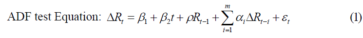
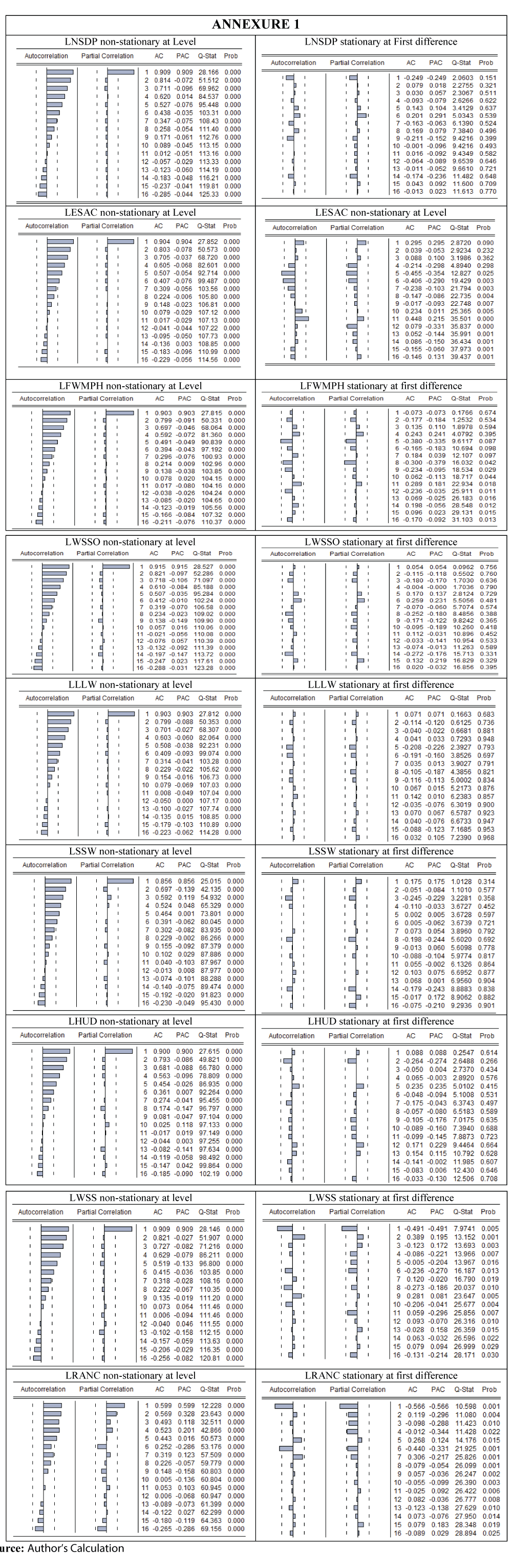
At the outset, all the transformed variables are checked for stationarity⁵. All the variables have been checked by various methods, viz., Augmented Dicky-Fuller (ADF) test (Equation 1), Phillips-Perron (PP) test (Equation 2), Kwiatkowski-Phillips-Schmidt-Shin (KPSS) tests (Equation 3). It is important to note that both ADF test and PP test are formulated to test the null hypothesis that the series is non-stationary, whereas the KPSS test is alternative to which has the null hypothesis is stationary. All the above tests suggest that all the variables are integrated of order, i.e., I (1) variables (Table 2). This means after the first difference they would become stationary or I (0) variables. The graphical representation of the stationary checking (using correlogram) is also given in Annexure 1. Since all the variable are I (1) we have tested the Granger causality (Engel, 1987); Granger, 1969) test (Equation 4) in the first difference form which is I (0) to avoid the likely spuriousness (Table 3). Moreover, a Johansen Co-integrating regression (Johansen, 1988) is also run using the I (1) series following Engel (1987) and Granger (1969) to find the long-run relationship (Equation 4 and Table 4).

Table 2: Unit Root Test Results
Variables	Stationarity Test Result
	At the Level form			First difference form
	Without trend and intercept	With intercept but no trend	With intercept and trend	Without trend and intercept	With intercept but no trend	With intercept and trend
Augmented Dickey Fuller (ADF) Test
LNSDP	7.8 (1.0)	0.9 (0.9)	-2.13 (0.5)	-1.06 (0.2)	-6.9 (0.0)	-7.13 (0.0)
LESAC	7.5 (1.0)	-0.9 (0.7)	-4.1 (0.01)	-1.9 (0.05)	-3.7 (0.00)	-3.7 (0.03)
LFWMPH	6.4 (1.0)	0.5 (0.9)	-4.3 (0.01)	-0.4 (0.4)	-5.7 (0.00)	-5.6 (0.00)
LHUD	3.5 (0.9)	0.5 (0.9)	-1.7 (0.7)	-3.6 (0.00)	-4.7 (0.00)	-4.8 (0.00)
LLLW	5.3 (1.0)	-1.3 (0.5)	-2.1 (0.5)	-2.7 (0.00)	-4.7 (0.00)	-4.9 (0.00)
LSSW	2.9 (0.9)	-2.04 (0.2)	-3.3 (0.07)	-3.4 (0.00)	-4.3 (0.00)	-4.5 (0.00)
LWSS	4.8 (1.0)	-0.3 (0.9)	-3.5 (0.07)	-0.9 (0.3)	-9.2 (0.00)	-9.02 (0.00)
LWSSO	3.4 (0.9)	0.8 (0.9)	0.1 (0.9)	-1.8 (0.6)	-4.8 (0.00)	-4.8 (0.00)
LRANC	1.1 (0.9)	-1.1 (0.7)	-6.8 (0.0)	-9.7 (0.00)	-9.9 (0.00)	-9.79 (0.00)
Phillips-Perron (PP) Test
LNSDP	9.6 (1.0)	1.3 (0.9)	-2.05 (0.5)	-2.4 (0.01)	-7.01 (0.00)	-7.2 (0.00)
LESAC	5.8 (1.0)	-0.8 (0.7)	-2.2 (0.4)	-1.7 (0.08)	-3.7 (0.00)	-3.7 (0.03)
LFWMPH	7.4 (1.0)	0.6 (0.9)	-2.2 (0.4)	-2.6 (0.01)	-5.7 (0.00)	-5.6 (0.00)
LHUD	6.4 (1.0)	0.9 (0.9)	-1.6 (0.7)	-3.6 (0.00)	-4.6 (0.00)	-6.4 (0.00)
LLLW	4.9 (1.0)	-1.4 (0.5)	-2.2 (0.4)	-2.5 (0.01)	-4.9 (0.00)	-4.8 (0.00)
LSSW	2.6 (0.9)	-2.06 (0.2)	-3.4 (0.07)	-3.3 (0.00)	-4.2 (0.00)	-4.5 (0.00)
LWSS	3.0 (0.9)	-0.02 (0.9)	-3.5 (0.05)	-5.8(0.00)	-9.03 (0.00)	-8.8 (0.00)
LWSSO	4.2 (1.0)	0.16 (0.9)	-1.8 (0.6)	-3.7 (0.00)	-4.8 (0.00)	-4.8 (0.00)
LRANC	1.9 (0.9)	-2.08 (0.2)	-14.5 (0.00)	-10.7 (0.00)	-31.1 (0.00)	-27.02 (0.00)
Kwiatkowski-Phillips-Schmidt-Shin (KPSS) Test
LNSDP	---	0.7 (0.4)	0.17 (0.14)	---	0.22 (0.46)	0.10 (0.14)
LESAC	---	0.7 (0.46)	0.05 (0.14)	---	0.08 (0.46)	0.06 (0.14)
LFWMPH	---	0.7 (0.46)	0.1 (0.14)	---	0.1 (0.46)	0.06 (0.14)
LHUD	---	0.7 (0.46)	0.6 (0.14)	---	0.1 (0.46)	0.07 (0.14)
LLLW	---	0.7 (0.46)	0.06 (0.14)	---	0.1 (0.46)	0.07 (0.14)
LSSW	---	0.7 (0.46)	0.06 (0.14)	---	0.2 (0.46)	0.11 (0.14)
LWSS	---	0.7 (0.46)	0.09 (0.14)	---	0.08 (0.46)	0.08 (0.14)
LWSSO	---	0.6 (0.46)	0.16 (0.14)	---	0.14 (0.46)	0.13 (0.14)
LRANC	---	0.7 (0.46)	0.5 (0.14)	---	0.32 (0.46)	0.32 (0.14)

Note: Entries in each cell shows Test Statistics and the probability of the Test Statistics is in the parentheses. In case of KPSS test 5% significant tabulated value of the test statics is in the parentheses.
Source: Authors? Calculation by using E-views software

Where, is the first difference of the is the intercept, are the coefficients, t is the time or trend variable, m is the number of lagged terms chosen to ensure that is white noise, i.e., contains no autocorrelation, is the pure white noise error term and is the sum of the lagged values of the dependent variable .

Phillips Perron Equation: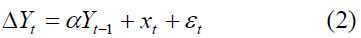

KPSS equation: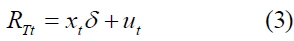

And α=ρ-1

LNSDP_t=Log of Net State Domestic Product in Haryana

LESAC_t=Log of expenditure on Education, Sports, Art & Culture

LFWMPH_t=Log of expenditure on Family Welfare, Medical & Public Health

LWSSO_t=Log of expenditure on Welfare of SC, ST & OBC

LLLW_t=Log of expenditure on Labour & Labour Welfare

LSSW_t=Log of expenditure on Social Security & Welfare

LHUD_t=Log of expenditure on Housing and Urban Development

LWSS_t=Log of expenditure on Water Supply and Sanitation

LRANC_t=Log of Relief on Account of Natural calamities

Results and Discussion

Descriptive Statistics

To know the nature of the variable this paper tested all the variabls by using descriptive statistics. Then it explains the trends and patterns of growth rate and social expenditure in the state of Haryana. The study have plotted the trends of growth rate of NSDP and growth rates of expenditures on various heads of social sector development., It has used to get an idea about the relationship between Net state Domestic Product (NDSP) and expenditures on social sector development in Haryana. However, the compound annual growth rate of social expenditure and NSDP of Haryana is e positive. It was 19.95 (Social Exp.) and 6.92 (NSDP) percent over the study period. Since most of the state is following the recent campaign of “Make in India⁶”, the state Haryana is not an exception. It is clear that in the recent years, particularly, since 2005 the growth rate of expenditures on social sector development is very high in Haryana. Though growth rate of NSDP is high during the last decade the growth rate of expenditure on social sector development is much higher than that of NSDP growth rate (Figure 1).

This could be due to the initiatives were taken in both 11^th and 12^th plan periods in order to achieve inclusive growth in India. Since the development of the social sector is indispensable for the achievement of inclusive growth in India. The government of Haryana has also spent substantially on education, healthcare, housing, sanitation and social security and labour welfare for the economic growth and development in Haryana. The result of the descriptive statistics found that though most of the variables do not follow the normal distribution, but they have low standard deviation and moderate skewness (Annexure 2). Furthermore, the high degree of correlation between NSDP with various expenditures on social sector development (Annexure 3) enables us for doing further econometrics analysis.

Econometrics Results

This study has used Granger causality test to find out the cause and effect relationship between NSDP and expenditure on social sector development in Haryana. This method explains about the short-run relationship among the variables which are included in this study. The causality test statistics suggest that NSDP causes the Family Welfare and Medical Facilities (FWMPH), Housing and urban development (HUD), the welfare of SC, ST&OBC (WSSO) and Relief on account of natural calamities (RANC). It indicates that there is a short run relationship between the same variable. But only one variable (Social Security Welfare) have an impact on NSDP (Table 3). This might have happened because of the fact that in the short-run, the government of Haryana could not able to spend on social sector development until 2005 (Figure 2). Furthermore, the increase of social sector development in Haryana could also be affected hugely by the central government schemes (social development schemes⁷) during the last decade, particularly, during the 11^th and 12^th five years periods. Hence the share of expenditure on social sector development was very high during that (post 2005) periods.

Because of the focus on inclusive development in the last decade and initiatives for “Make in India” in recent years. It is expected that both the growth of NSDP and social sector expenditure would increase further in long-period. And more importantly, the increasing expenditure on social sector development would increase labour productivity through skill development. This skill development programmer would encourage people (those who belong to women and socially marginalized groups including Muslims) to participate in labour market. Increament of labour force participation in labour market leads to increase parcapita income and standard of living which leads to growth of NSDP in Haryana. It is clear from the results of Johansen co-integration that growth of NSDP and social sector expenditure are significantly related in the long-run i.e. there is a long-run relationship between NSDP and social expenditure in Haryana. Both Johansen’s Trace statistics and Maximum Eigen value test suggests that there exists six significant (at 5% level) co-integrating relations (Table 3). This implies the fact that in the long run NSDP and social sector development are inter-dependent and would cause each other.

Table 3: Granger Causality Test Results
Null Hypothesis	F-Statistic	Prob.
Causality between NSDP and Exp. On Education, Sports, Art & Culture
ESAC does not Granger Cause NSDP	1.47612	0.2485
NSDP does not Granger Cause ESAC	2.56358	0.0979
Causality between NSDP and Exp. On Family welfare & Medical facilities
FWMPH does not Granger Cause NSDP	0.01656	0.9836
NSDP does not Granger Cause FWMPH	3.68726	0.0401
Causality between NSDP and Exp. On Housing & Urban development
HUD does not Granger Cause NSDP	0.60846	0.5524
NSDP does not Granger Cause HUD	4.92423	0.0161
Causality between NSDP and Exp. On Labour & Labour welfare
LLW does not Granger Cause NSDP	2.56176	0.0981
NSDP does not Granger Cause LLW	2.14206	0.1393
Causality between NSDP and Exp. On Water supply and Sanitation
WSS does not Granger Cause NSDP	0.98816	0.3869
NSDP does not Granger Cause WSS	1.02539	0.3738
Causality between NSDP and Exp. On welfare of SC,ST&OBC
WSSO does not Granger Cause NSDP	0.41101	0.6676
NSDP does not Granger Cause WSSO	4.51779	0.0216
Causality between NSDP and Exp. On Social Security Welfare
SSW does not Granger Cause NSDP	7.87816	0.0023
NSDP does not Granger Cause SSW	28.6137	4.007
Causality between NSDP and Relief on account of natural calamities
LRANC does not Granger Cause LNSDP	1.89986	0.1714
LNSDP does not Granger Cause LRANC	7.76846	0.0025
Number of Observations	29

Source: Author?s Calculation

Table 4: Johansen Co-Integration Results
Hypothesized No. of CE(s)	Eigenvalue	Trace Statistics (#)	Critical Value at 5% (p-value)	Maximum Eigen Statistics ($)	Critical Value at 5% (p-value)
None	0.989936	445.79*	197.37 (0.000)	133.36*	58.43 (0.00)
At most 1	0.960702	312.42*	159.53 (0.000)	93.86*	52.36 (0.00)
At most 2	0.915105	218.56*	125.61 (0.000)	71.52*	46.23 (0.00)
At most 3	0.874540	147.03*	95.75 (0.000)	60.19*	40.07 (0.00)
At most 4	0.640992	86.84*	69.81 (0.000)	29.70	33.87 (0.14)
At most 5	0.612767	57.13*	47.85 (0.005)	27.51	27.58 (0.05)
At most 6	0.485702	29.61	29.79 (0.032)	19.28	21.13 (0.08)
At most 7	0.299610	10.33	15.49 (0.205)	10.32	14.26 (0.19)
At most 8	0.000254	0.007	3.84 (0.069)	0.00	3.84 (0.93)

*denotes rejection of the hypothesis at the 0.05 level
# Trace test indicates 6 co-integrating equations at the 0.05 level
$ Max-eigenvalue test indicates 4 co-integrating equations at the 0.05 level
Source: Authors Calculation.

Concluding Remarks

In the context of inclusive growth and “Make in India” initiatives of the central government. The role of the state government of Haryana becomes very important for initiating various developmental strategies for the all-round development of the state. In the recent years, an increase in the public spending on various heads of social development has increased in Haryana. This paper examines both short-run and long-run relationship between economic growth and social sector development through human capital formation in Haryana. The major findings of the paper show that increased expenditure on social sector development has a strong and positive impact on growth of NSDP in Haryana. The results of the study also show that a significant relationship between growth and social sector development in the short-run (Granger causality result is significant). However, it suggests a long-run positive relation between the two (Johansen co-integration). The Ganger causality test identified that expenditure on some social factors is positively significant towards economic growth. Expenditure on Social Security Welfare (SSW) unidirectional (only) and others are statistically insignificant. Though govt. of Haryana invested for social sector development but it does not reach to the poor section of the people who are in root in the economy.

Therefore, Govt. of Haryana should focus on public investment in human capital i.e. expenditure on social sector development that will encourage to the growth of the economy.

Endnotes

1. It comprising of sub-sectors like education, health and medical care, housing, sanitation and water supply, etc.

2. Per capita income refers to the average income earned per person in a given area in a particular period of time. It is calculated by dividing the total income by total population.

3. Real per capita is adjusted with the inflation in a specific period of time.

4. When the variance of the residual is not constant, it makes difficult to precisely test the null hypothesis. For detail see Gujarati (2007), 3^rd edition, chapter 11, p: 396-449.

5. A variable is said to be strongly stationary if its mean and variances are constant over the years and the covariance at each lag is constant. And it would be weak stationary if its mean and variances are constant over the years and the covariance at a constant lag is constant. For detail see Enders (2004).

6. Make in India, a type of Swadeshi movement covering 25 sectors of economy, was launched by the Government of India in 2014 to encourage companies to manufacture their products in India.

7. Sarva Shiksha Abhiyan (SSA) and Rashtriya Madhyamik Shiksha Abhiyan (RMSA) National Skills Qualifications Framework (NSQF), National Rural Health Mission (NRHM), Janani Shishu Suraksha Karyakram (JSSK), Janani Suraksha Yojana (JSY - GOI), Mukhiya Mantri Muft Ilaj Yojana (MMIY), Mukhya Mantri Anusuchit Jaati Nirmal Basti Yojana (MMAJNBY), Rural housing yojana like Priyadarshini Awaas Yojana (PAY), MGNREGS, Indiara Awas Yojana (IAY), National Rural Livelihood Mission (HSRLM), Rajiv Awas Yojana (RAY), Integrated Housing & Slum Devlopment Programme (IHSDP) and Swaran Jayanti Shahari Rozgar Yojana (SJSRY).

References

1. Sen, A. (1989). Development as capability expansion. In Sakiko FukudaParr and A K Sivakumar (eds). Readings in Human Development, 3-13.
2. Baldacci, E., Clements, B., Gupta, S. & Cui, Q. (2008). Social spending human capital and growth in developing countries. World Development, 36(8), 1317-1341.
3. Benhabib, J. & Spiegel, M.M. (1994). The role of human capital in economic development: Evidence from cross-country data. Journal of Monetary Economics, 34(2), 143-173.
4. Bhat, R. & Jain, N. (2004). Analysis of public expenditure on health using state level data. Indian Institute of Management Ahmedabad.
5. Culter, D., Deaton, A. & Lleras-Muney, A. (2005). The Determinants of Mortality, Working Paper, No. 11963. National bureau of economic research, Cambridge.
6. Datt, G. & Ravallian, M. (1998a). Why have some Indian states done better than others at reducing rural poverty? Economica, February, 65(257), 17-38.
7. Dickey, D.A. & Fuller, W.A. (1979). Distribution of the estimators for autoregressive time series with a unit root. Journal of the American Statistical Association, 74(366), 427-431.
8. Duflo, E. (2001). Schooling and labour market consequences of school contruction in Indonesia: Evidence from an unusual policy experiment. American Economic Review, 91(4), 795-813.
9. Enders, W. (2004). Applied econometric time series. Wiley, Second Edition.
10. Engle, R.F. & Granger, C.W. (1987). Co-integration and error correction: Representation, estimation and testing. Econometrica, 55, 251-276.
11. Gangal Vijay L.N. & Gupta, H. (2013). Public expenditure and economic growth a case study of India. Global Journal of Management and Business Studies, 3(2), 191-196.
12. Gbesemete, K.P. & Gerdtham, U.G. (1992). Determinants of health care expenditures in Africa: A cross-sectional study. World Development, 20, 303-308.
13. Goldstein, J.S. (1985). Basic human needs: the plateau curve. World Development, 13(5), 595-609.
14. Granger, C.W.J. (1969). Investigating causal relations by econometric models and cross spectral methods. Econometrica, 37, 424-438.
15. Grossman, G. & Helpman. (1991). Innovation and growth in the global economy. Cambridge, MIT Press.
16. Gujarati. (2007). Basic econometrics. Tata McGraw-Hill Education, 3rd edition, chapter 11, 396-449.
17. Haddad, L., Alderman, H., Appleton, S., Song, L. & Yohannes, Y. (2003). Reducing child malnutrition: How far does income growth take us? World Bank Economic Review, 17(1), 107-131.
18. Haldar, S.K. & Mallik, G. (2006). Does human capital cause economic growth? A case study of India. International Journal of Economic Sciences and Applied Research, 3(1), 7-25
19. Hicks, N.L. (1979). Is there a trade-off between growth and basic needs? Finance and Development, 17(2), 17-20.
20. Hitris T. & Posnett J. (1992). The determinants and effects of health expenditures in developed countries. Journal of Health Economics, 11, 173-181.
21. Hooda, S.K. (2013). Changing pattern of public expenditure on health in India: Issues and challenges. ISID-PHFI Collaborative Research Centre, Working Paper.
22. Johansen, S. (1988). Statistical analysis of co-integration vectors. Journal of Economic Dynamics and Control, 12, 231-254.
23. Kwiatkowski, D., Phillips, P.C.B., Schmidt, P. & Shin, Y. (1992). Testing the null hypothesis of stationary against the alternative of a unit root. Journal of Econometrics, 54, 1-3, 159-178.
24. Lucas, R. (1988). On the mechanics of economic development. Journal of Monetary Economics, 22(1), 3-42.
25. Mahal. & Ajay. (2000). Diet-linked chronic illness in India, 1995-1996: Estimates and economic consequences. Draft. New Delhi: National Council for Applied Economic Research.
26. Mankiw, G.N., Romer, D. & Weil, D. (1992). A contribution to the empirics of economic growth. Quarterly Journal of Economics, 107(2), 407-437.
27. Mohapatra, A.K. (2013). Enhancing human capabilities and augmenting economic growth through social sector development. Asian-African Journal of Economics and Econometrics, 13(2), 339-354.
28. Nelson, R. & Phelps, E. (1966). Investment in humans, technological diffusion and economic growth. American Economic Review, 5(2), 69-75.
29. Perron, P. (1989). The great crash, the oil price shock and the unit root hypothesis. Econometrica, 57(6), 1361-1401.
30. Quah, D. & Rauch, J.E. (1990). Openness and the rate of economic growth. Mimeo University of California, San Diego.
31. Ram, R. (1985). The role of real income level and income distribution in fulfilment of basic needs. World Development, 3(5), 589-594.
32. Rivera-Batiz, L.A. & Romer, P.M. (1991). Economic integration and endogenous growth. Quarterly Journal of Economics, May.
33. Romer P.M. (1989). Capital accumulation in the theory of long run growth. In Barro R.J. (ed.), Modern Business Cycle Theory.
34. Romer, P. (1986). Increasing returns and long-run growth. Journal of Political Economy, 94(5), 1002-1037.
35. Romer, P.M. (1990). Endogenous technological change. Journal of Political Economy, 98.
36. Schultz, T.P. (1997). Assessing the productive benefits of nutrition and health: anintegrated human capital approach. Journal of Econometrics, 77(1), 141-158.
37. Schultz, T.P. (2000). Productive benefits of improving health: Evidence from low income countries. Yale University Mimeo.
38. Sen, A. (2000). A decade of human development. Journal of Human Development, 1(1).
39. Strauss, J. & Thomas, D. (1995). Human resources: empirical modelling of households and family decisions. In J. Behrman and T.N. Srinivasan (Eds.): Hand Book of Development Economics, 3A, 1883-2023, Elsevier, Amsterdam.
40. Strauss, J. & Thomas, D. (1998). Health, nutrition and economic development. Journal of Economic Literature, 36(2), 766-817.
41. Streeten, P. (1981). First things first. Oxford University Press, London.
42. UNDP. (1990). Human Development Report, Oxford University Press.

Annexure 2: Descriptive Statistics
Statistics	LNSDP	LESAC	LFWMPH	LHUD	LLLW	LSSW	LWSS	LWSSO	LRANC
Mean	13.46	9.45	8.03	6.87	6.27	8.11	8.15	6.19	6.46
Median	13.36	9.50	8.03	6.49	6.30	8.24	8.17	5.83	6.77
Maximum	14.51	11.33	9.95	10.02	7.81	10.16	10.41	8.12	8.92
Minimum	12.55	7.35	6.34	4.60	4.37	4.98	5.92	4.70	3.30
Std. Dev.	0.62	1.23	1.11	1.75	1.07	1.41	1.46	1.14	1.40
Skewness	0.24	0.03	0.16	0.58	-0.06	-0.30	-0.17	0.45	-0.28
Kurtosis	1.78	1.86	1.93	2.10	1.88	2.57	1.76	1.76	2.29
Jarque-Bera	2.22	1.69	1.63	2.77	1.64	0.69	2.13	3.03	1.06
Probability	0.33	0.43	0.44	0.25	0.44	0.71	0.34	0.22	0.59
Sum	417.11	292.82	249.00	213.11	194.46	251.45	252.76	192.01	200.14
Sum of square deviation	11.42	45.21	37.19	91.56	34.56	59.76	63.83	39.22	58.87
Observations	31	31	31	31	31	31	31	31	31

Source: Author?s Calculation

Annexure 3: Pearson’s Coefficients Of Correlation
Variables	LESAC	LFWMPH	LHUD	LLLW	LSSW	LWSS	LWSSO	LRANC
LNSDP	0.99	0.99	0.98	0.98	0.97	0.97	0.98	0.86
Sig. (2-tailed)	0.000	0.000	0.000	0.000	0.000	0.000	0.000	0.00

Correlation is significant at the 0.01 (2-tailed)
Source: Authors Calculation.