Keywords

Cointegration, Granger-Causality, Impulse, Oilseeds, Stationary, VAR.

Abbreviations

NBE: the National Bank of Ethiopia CSA central statistical agency

ARCH: Autoregressive Conditional Heteroskedasticity

ARIMA: Autoregressive Integrated Moving Average

GARCH: Generalized Autoregressive Conditional Heteroskedasticity

GED: General Error Distribution

Background

Oilseeds are the most important agricultural commodities in the world. From 1998 to 2002, the average world oilseed production was 312 million metric tons per year. Oilseeds Consumption was found to be the most elastic to both price and production (Mattson et al., 2004). About 60% of the world's sesame production was from Myanmar, India, China, Ethiopia, and Nigeria during 2011 and Ethiopia is among the top 5 world's producers of a sesame seed, linseed, and Niger seed (Ayana, 2015). The country produces different types of oilseeds varieties such as sesame seed, linseed, Niger seed, sunflower seed, soybeans, cottonseed, and rapeseed. From these, sesame seed, linseed, and Niger seed are the major export crops (Yifru, 2015).

The Ethiopian oilseed sector has several strengths like a large diversity of high-value oilseeds crops, significant world production in sesame seed, linseed, and noug. However, it has a weak side like lacking sufficient international market orientation, high transaction costs due to a large number of chain actors, and weak farm production (Wijnands et al., 2009).

Ethiopia's oilseed sector plays a very important economic role in generating foreign exchange earnings and income for the country. One-fifth of Ethiopia's total export earnings are generated from oilseeds exports, with sesame being the second-largest export revenue after coffee. The higher prices at several markets are indeed challenging. As Ethiopia is the 5^th world producer of linseed, export opportunities should be further explored. Niger seed exports account for a third of Ethiopia's American exports (Wijnands et al., 2007). The study of (Kefyalew, 2012) was focused on the production-related problem of this crop, but they couldn’t see the export and domestic price of the crop. Also (Sebsib & Emmanuel, 2018) studies export price volatility of Sesame only, ignoring domestic price and production of oilseeds. But, the interdependence among the production, domestic price, and export price of oilseeds was not yet investigated.

Generally, this study explores the relationship between production, domestic price, and export price of oilseeds in Ethiopia from January 2002 to December 2016 by using vector autoregressive time series analysis. More specifically to fit appropriate multivariate time series model, to examine the extent of their relation, to identify the factors that have a significant effect.

Methods

Data for the Study

In this study, we have considered secondary data on annual production, monthly domestic and export price of oilseeds, monthly Exchange rate, monthly inflation rate, monthly fuel oil price, and annual GDP in Ethiopia. All these data were from CSA and the National Bank of Ethiopia (NBE) over the period from January 2002 to December 2016. The data we get for production and GDP are annual but in this study, it converts to monthly data by using views software.

Variables Considered in the Study

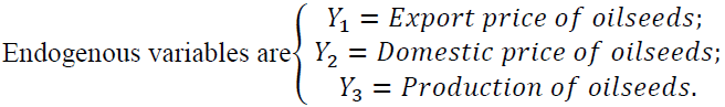
In this study export price, domestic price, and production of oilseeds are considered as dependent variables or endogenous variables.

The Lag of endogenous variables can also be independent variables like export price, domestic price, and production of oilseeds, and all the exogenous variables such as inflation rate, exchange rate, price of fuel oil, and GDP are considered as independent variables. An inflation rate is a rate at which prices increase over time and resulting in a fall in the purchasing value of money, a higher inflation rate is not good for the economy. Also, the exchange rate is defined as the conversion of one currency to another, in this study exchange rate is the conversion of the US dollar to ETB. The total value of everything produced by all the companies and people in the country is measured by GDP.

Data Analysis

In this, the study multivariate time series model is appropriate to analyze the interdependence between production, domestic price, and export price of oilseeds. VAR model is a specific subset of multivariate modeling.

Vector Autoregressive (VAR) Models

VAR model was introduced by (Sims, 1980) as a technique that could be used by macro-economists to characterize the joint dynamic behavior of a collection of variables without requiring strong restrictions of the kind needed to identify underlying structural parameters. Since this paper concerns the relationship between the production of oilseeds, domestic and export price of oilseeds multivariate time series is appropriate instead of univariate time series.

The VAR model is particularly important since viewed as a system of reduced-form equations in which each of the endogenous variables is regressed on its own lagged values and the lagged values of all other variables in the system (Gujarati, 2004).

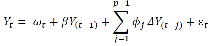
VAR model consists of a set of 7 variables from which 3 variables are endogenous and the remaining 4 are exogenous variables. be 3-dimensional endogenous variables and be exogenous variables, observed at time months and defined with order as shown in Equation 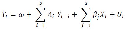1.

(1)

Where is a 3-dimensional constant vector, the and are and coefficient matrices respectively for matrices and is dimensional Gaussian process with and time-invariant positive definite covariance matrix . In this case indicates export price of oil seeds, domestic price of oil seeds and production of oil seeds, observed from 2002 to 2016 and indicates the order of integration up to.

In the VAR process, each of the time-series data under study should be stationary. That is, there is a need to test for stationary of the series, which is also called the unit root test. An information criterion is used to find the model that fits the data well from a group of models. Three criteria functions are commonly used to determine VAR order. Under the normality assumption, these three criteria for a VAR( ) model are: AIC, the Akaike information criterion proposed by (Akaike, 1981), BIC stands for Bayesian information criterion (Schwarz, 1978) and HQ( ) is proposed by (Hannan & Quinn, 1979).

The additional test of after the estimation of the VAR(P), Granger Causality, cross correlation, normality and Heteroskedasticity is checked.

In forecasting the estimated VAR model, an impulse response function was used to see the effect of a one-time shock to one of the innovations on current and future values of the endogenous variables through the dynamic lag structure of the VAR model estimation. Also, the variance decomposition method was applied to measure the percentage of the forecast error variances at various forecast horizons that are attributable to each of the individual shocks.

Co-Integration Test

After testing the stationary of the variables and selection of the VAR order it is important to know the order of integration before discussing the existence of a relationship among variables either in the short or long term. The likelihood ratio (LR) test and the trace test are the best-known approaches to co-integration tests for VAR models (Johansen, 1991). Consider the extended Gaussian VAR (p) model with a trend component in Equation 2 given by

(2)

Where is a deterministic term and is the matrix that plays the most important role in the co-integration study.

A Vector Autoregression (VAR) model expresses each variable as a linear function of its past values, the past values of all other variables that are considered in the study, and a serially uncorrelated error term.

Granger Causality Test

In multivariate time series analysis, it is important to know which variable causes another variable by using a causality test. Granger causality is a technique for determining whether one series is useful in forecasting another. A variable Y is causal for another variable X if knowledge of the history of Y is useful for predicting the future state of X over and above the knowledge of the past history of X itself (Grange, 1969).

The model checking plays an important role in model building to ensure that the fitted model is adequate or not. After a VAR model has been estimated, we must check for the absence of serial correlation and Heteroskedasticity. Also, it is important to check if the error process does not violate the distributional assumption, multivariate normality. For testing the lack of serial correlation in the residuals of a VAR (p)-model, a Portmanteau test and the Lagrange multiplier (LM) test are used (Breusch, 1978; Godfrey, 1978).

Forecasting

After a VAR model has been estimated and passes the diagnostic tests, it is suitable to be used for forecasting. Future observations are recursively forecasted using the VAR (p) model for time horizon according to (Box et al., 2008) and (Pfaff, 2008) as shown in Equation 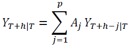3

(3)

In addition to Granger causality, there is another approach to explore the relationship between variables is called impulse response functions.

Forecast Error Variance Decompositions

Forecast error variance decompositions (FEVD) show the portion of the variance in the forecast error for each variable due to innovations to all variables in the system (Enders, 1995). The main objective of FEVD is to achieve information about the forecast ability. That means even a perfect model involves ambiguity about the realization of due to uncertainty in the associated error terms. The FEVD answers the type of question: what portion of the variance of the forecast error in predicting is due to the structural shock? Using the orthogonal shocks in equation 4 the h-step ahead forecast error vector, with known VAR coefficients, may be expressed as shown in Equation 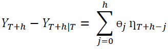4.

(4)

In particular for this forecast error has the form expressed as shown in Equation 5

(5)

The variance of the h-step forecast of the orthogonal structural error is expressed as shown in Equation 6

(6)

Where Pfaff (2011); Tsay (2005).

The portion of due to shock is then

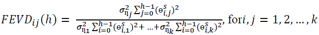(7)

In a VAR with variables, there would be values. The FEVD in Equation 7 depends on the recursive causal ordering used to identify the structural shocks and is not unique. We must understand that different causal orderings would produce different FEVD values.

Results

Data

The data sets in this study consist of the monthly export price of oilseeds (in ETB per kg), monthly domestic price of oilseeds (in ETB per kg), monthly production of oilseeds (in quintal), monthly inflation rate, monthly exchange rate (in ETB against US dollar), monthly GDP (in millions of birr) and monthly price of fuel oil (in ETB per metric ton) in Ethiopia from January 2002 to December 2016. The average domestic price of oilseeds is 20.79 birr per kg. The observed data also shows that the average monthly export price and product of oilseeds was 23.29 birr per kg and 6089498 quintals, respectively in Table 1.

Table 1 Descriptive Statistics for all Endogenous and Exogenous Variables
	Exppric	Domstpric	Product	Infn rate	Exng rate	Price fo	Gdp
Mean	23.29	20.79	6089498	14.05	14.08	47586.96	386086.5
Median	20.86	20.01	6465667	10.09	10.34	7337.07	274481
Maximum	48.98	59.50	8728241	64.16	23.72	756873	989736
Minimum	2.12	3.98	1919969	-7.34	8.47	171.04	61117.45
Skewness	-0.02	0.35	-0.94	1.62	0.44	3.43	0.63
Kurtosis	1.64	2.44	3.16	5.93	1.48	14.59	1.83
Jarque-Bera	13.83	5.98	26.70	143.51	23.13	1360.87	22.07
Probability	0.000994	0.040346	0.000002	0.000000	0.000009	0.000000	0.000016

Test of Stationarity of the Data

The time plot of the graph shows that the export price, domestic price, and production of oilseeds continuously increase or have an upward trend which means time series data is non-stationary we can see from Figure 1.

Also, the time plots of all the exogenous variables are non-stationary in Figure 2. In addition to this checking Stationery without trend at the level by using ADF and PP tests indicates almost all the variables are non-stationary indicated in Table 2. So, it is necessary to look for possible transformations that might bring stationary. The transformation of the data using the logarithmic and differencing method. After the first difference of logarithm, the variables of each series become stationary at a 5% level of significance which means each series is integrated of order one? The macroeconomic time series variables are regarded stationary at first difference, integrated of order one, i.e. I(1) we can found in Table 3.

Table 2 Unit Root Test of Stationarity without Trend at 5% Level of Significance
Variables	ADF	PP	Status
Stationarity at Level
Exp. price	-4.009463(0.0100)	-8.570773(0.0000)	I(0)
Domst. price	-7.309728(0.0000)	-6.991585(0.0000)	I(0)
Product	-3.190976(0.0896)	-2.495193(0.3302)	I(0)
In flation rate	-4.105656(0.0074)	-2.914140(0.1606)	I(0)
Exchange rate	-2.534466(0.3113)	-4.860969(0.0005)	I(0)
Fuel oil price	-2.773414(0.2092)	-4.927592(0.0004)	I(0)
GDP	-2.325253(0.4178)	-2.089794(0.5476)	I(0)
Stationarity at first difference of the log transformed
Product	-4.087296(0.0079)	-9.354244(0.0000)	I(1)
Infl ation rate	-7.179599(0.0000)	-7.388115(0.0000)	I(1)
Exchange rate	-15.71552(0.0000)	-42.37011(0.0001)	I(1)
Fuel oil price	-15.49176(0.0000)	-20.41256(0.0000)	I(1)
GDP	-13.22273(0.0000)	-13.22273(0.0000)	I(1)
t-Statistic (P-value)

Table 3 Unit Root Test of Stationarity with Trend at 5% Level of Significance
Variables	ADF	PP	Status
at Level of Log Transformed
Log exp. price	-3.710645(0.0047)	-2.345953(0.1589)	I(0)
Log domst. price	-1.281076(0.6380)	-1.476499(0.5434)	I(0)
Log product	-2.139601(0.2296)	-2.007857(0.2833)	I(0)
Infl ation rate	-4.138961(0.0011)	-2.984399(0.0383)	I(0)
Exchange rate	-0.099081(0.9467)	-0.541448(0.8789)	I(0)
Fuel oil price	-2.704836(0.0752)	-4.848559(0.0001)	I(0)
at First Difference of Log Transformed
d1Logexp. Price	-15.42561(0.0000)	-31.83188(0.0001)	I(1)
d1Logdomst. Price	-10.33063(0.0000)	-39.49648(0.0001)	I(1)
d1Logproduct	-3.709309(0.0047)	-8.771263(0.0000)	I(1)
d1 exchange rate	-15.70563(0.0000)	-37.68364(0.0001)	I(1)
d1fuil oil price	-15.53220(0.0000)	-20.46762(0.0000)	I(1)
d1GDP	-13.23617(0.0000)	-13.23617(0.0000)	I(1)
t-Statistic (P-value)

Tests for Autocorrelation

The correlation between the endogenous variables is at a 5% level of significance all the correlation coefficients are an approach to 1 which means a strong correlation between the endogenous variables. Since the endogenous variables are highly correlated multivariate time series analysis is quite reasonable instead of univariate time series model we can see Table 4.

Table 4 Correlation Matrix for all Endogenous Variables
Correlation coeffi cient (probability)	Export price	Domestic price	Product
Export price	1.000000	0.879142(0.0000)	0.876321(0.0000)
Domestic price	0.879142(0.0000)	1.000000	0.866361(0.0000)
Product	0.876321(0.0000)	0.866361(0.0000)	1.000000

Order Selections of VAR Model

An information criterion is used to find the model that fits the data well. The results show that Schwarz Bayesian information Criterion is minimum at lag 2, and the Akaike information criterion and Hannan-Quinn information criterion are minimum at lag 4. Thus the SBIC criteria select a VAR (2) while AIC and HQ criteria select a VAR (4) model, but we take the joint optimum lag length of order two VAR (2) we can see in Table 5.

Table5 Var Order Selection by Different Selection Criteria
Lag	AIC	SBIC	HQ
0	-0.534607	-0.259023	-0.422787
1	-6.224538	-5.783603	-6.045625
2	-6.463471	-5.857185*	-6.217466
3	-6.583921	-5.812285	-6.270824
4	-6.687682*	-5.750695	-6.307492*
5	-6.682023	-5.579685	-6.234741
6	-6.684610	-5.416921	-6.170236
7	-6.618183	-5.185143	-6.036716
8	-6.615103	-5.016713	-5.966544

Co-Integration Test

These methods allow us to test the existence of a long-term relationship between the dependent and the explanatory variables in a multivariate framework. The null hypothesis claims no co-integration is rejected at the conventional level of significance, since the trace test statistic and rank test (maximum Eigenvalue) is greater than the critical value at all co-integrating vectors, or we have a significant probability value to both trace test and maximum Eigenvalue that is 0.0130 and 0.0413, respectively. That is, both the trace statistic and the maximum Eigenvalue indicates the existence of at least one co-integrating vector at a 5% level of significance. Thus, there is one co-integrated vector in the system. So, we have enough evidence to conclude that there exists a long-run relationship among the variables. This is equivalent to say among d1log export price, d1log domestic price, and d1log production of oilseeds, there is one long-run relationship in Table 6.

Table 6 Result of Johansen Co-Integration Test
Null hypothesis	Alternative hypothesis	Eigen value	Statistic	5% critical value	Prob.
Trace test()
		0.115473	34.58372	29.79707	0.0130
		0.062098	12.86546	15.49471	0.1198
		0.008540	1.518075	3.841466	0.2179
Maximum Eigen value test()
		0.115473	21.71826	21.13162	0.0413
		0.062098	11.34738	14.26460	0.1377
		0.008540	1.518075	3.841466	0.2179

Estimation of VAR Model

After determining the variable's co-integration and long-run relationship between the variables, we are going to estimate a VAR model. The main target of this study is to assess the dependency of current values of the first difference of the log-transformed endogenous variables (production, domestic, and export price of oilseed) own past values, on the past values of other variables, and the exogenous variables.

As we see from Table 7 d1log export price of oilseeds is negatively related to its own first and second lags, first lag of d1log production of oilseeds, d1exchange rate, d1 fuel oil price, and d1 GDP but positively related to both first and second lag of d1log domestic price of oilseeds, second lag of d1log production of oilseeds and d1 inflation rate. Also, d1log Domestic price of oilseeds is positively related to the second lag of d1log production of oilseeds, d1 exchange rate, d1 fuel oil price, d1 GDP and negatively related to the first two lags of d1log export price of oilseeds, its own first two lags, the first lag of d1log production of oilseeds and d1 inflation rate. The d1log Production of oilseeds is related with the first two lags of d1log export price of oilseeds, the second lag of d1log domestic price of oilseeds, its own first two lags, d1 exchange rate, d1 fuel oil price, and d1 GDP positively and it is negatively related with the first lag of d1log domestic price and d1 inflation rate.

Table 7 Results of Parameter Estimates of Fitted Var (2) Model
Lags of variables	d1logexport price	d1logdomestic price	d1logproduct
c	0.011447 (0.6113)	0.023573 (0.2445)	0.004518(0.0342)
d1logexport price(-1)	-0.600831 (0.0000)	0.120717 (0.0463)	0.000895(0.8960)
d1logexport price(-2)	-0.313998 (0.0000)	-0.121892 (0.0611)	0.006084(0.3733)
d1logdomestic price(-1)	0.092884 (0.2495)	-0.302888(0.0000)	-0.006872(0.3673)
d1logdomestic price(-2)	0.027001(0.7384)	-0.217402 (0.0029)	0.008034 (0.2935)
d1logproduct(-1)	-0.047098 (0.9513)	-2.096101 (0.0026)	0.360170 (0.0000)
d1logproduct(-2)	1.533272 (0.0467)	2.425636  (0.0005)	0.280015 (0.0001)
Inflation rate	0.000265 (0.8088)	-0.000380 (0.6990)	-0.000112(0.2806)
d1 exchange rate	0.024496 (0.0245)	0.011271 (0.0253)	0.000208 (0.8421)
d1fuil oil price	1.41x10-7(0.0379)	1.11x10-7(0.4393)	9.21x10-9(0.5421)
d1gdp	-3.28x10-5(0.0035)	4.59x10-6(0.6481)	2.16x10-6(0.0419)
R-squared	0.534575	0.414001	0.459029
Adj. R-squared	0.494489	0.366651	0.420416
F-statistic	8.346446	4.519613	9.298200

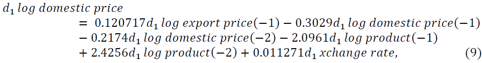
VAR (2) model is fitted with the variables whose lag coefficients are significant. From the results of the fitted model in Table 7. When we consider the d1log export price of oilseeds, d1log domestic price of oilseeds, and d1log production of oilseeds as the dependent (endogenous) variable the equation of the fitted model in Equations 8-10, respectively becomes

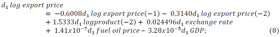
About 49.45%, 36.67%, and 42.04% of the variation of d1log export price, d1log domestic price, and d1log product of Ethiopian oilseeds are explained by the given explanatory variables respectively.

Similarly one month last of the d1log export price of oilseeds, two months last of oilseeds d1log product and d1 exchange rate affect d1log domestic price of oilseeds positively. Adjusted R square indicates that 36.66% variation of Ethiopian d1log domestic price of oilseeds expressed by the variables included in this study. Also, the d1log production of oilseeds is affected by positively its one-month and two-month lags and gross domestic product in Ethiopia and about 42.04% variation is explained by the variables included in this study. The other variables included in this study have no effects on the production of oilseeds in Ethiopia.

Granger Causality Test

The Granger causality test is a useful technique for determining whether one series is good for forecasting the other. From Table 8 results of multivariate Granger causality tests, we observe that d1log production of oilseeds granger causes to d1log domestic price of oilseeds (F-test statistic of 6.9306 and p-value of 0.0013) and this indicates a unidirectional causality from d1log production to d1log domestic price of oilseeds. This implies that the change in d1log production of oilseeds leads to a change in the d1log domestic price of oilseeds. That is, d1log production of oilseeds provides important information to forecast the future value of the d1log domestic price of oilseeds. Reject the null hypothesis that one variable does not Granger-cause to the other variable. For example, d1log export price of oilseeds does not Granger-cause of d1log production of oilseeds, and also d1log domestic price of oilseeds does not Granger-cause d1log production of oilseeds and d1log export price of oilseeds in Ethiopia.

Table 8 Granger Causality Test for Fitted Var (2) Model
Null Hypothesis	Obs	F-Statistic	Prob.
d1ldomestic price doesn't Granger Cause d1lexport price	177	0.39703	0.6729
d1lexport price doesn't Granger Cause d1ldomestic price	177	1.81085	0.1666
d1lproduct doesn't Granger Cause d1lexport price	177	2.19463	0.1145
d1lexport price doesn't Granger Cause d1lproduct	177	0.89075	0.4122
d1lproduct doesn't Granger Cause d1ldomestic price	177	6.93060	0.0013
d1ldomestic price doesn't Granger Cause d1lproduct	177	1.41248	0.2463

The diagnostic test of the model to check the assumed model may not be a good approximation to reality. So, the fitted model is adequate and has the desired econometric properties that are it has correct functional form since the residuals are serially uncorrelated, homoscedastic, and multivariate normal shown in Table 9.

Table 9 Diagnostic Test for Fitted Var (2) Model
Test	Q-Stat	df	Prob.
Portmanteau(serial autocorrelation)	11.6646	18	0.8583
JarqueBera-VAR(Multivariate normality)	3.5043	180	0.1734
VAR Residual Heteroskedasticity Tests	1.67319	6	0.9472

Forecasting

In Figure 3 when we look at forecasting of in sample d1log export price of oilseeds, at the beginning it changes slowly, but between 2011 and 2013 there was a high fluctuation and after 2013 it varies slowly. While the d1log domestic price of oilseeds had a high variation at the beginning, that is, between 2002 and 2007 and after this time the variation is small. The bottom figure indicates the forecasted value of d1log production of oilseeds, it shows that there was a sudden fluctuation between 2002 and 2012 but after 2012 almost it becomes a small variation.

Impulse Response Functions of Fitted VAR (2) Model

In this study, the VAR model permits to study of the impulse response of endogenous variables (export price, domestic price, and production of oilseeds) to the one-time shock of other variables in the model. In Figure 4 from the left 3 Figures, we observe that one positive shock to d1log export price of oilseeds leads to a positive response from its own, positive response from d1log domestic price and stable from d1log product of oilseeds in the lower lags until period 1, 1 and 2 respectively; but after this period as d1log export price changes by one positive shock the response from its own, d1log domestic price and d1log product of oilseeds is negative, negative and positive until period 3, 3 and 4 respectively and after this period these are changed to positive, positive and almost stable response in the lower lags. In the higher lags as d1logexport price of oilseeds changes by one-time shock, it leads stable response from all variables.

In Figure 4 from the middle 3 figures we observe that one positive shock to d1log domestic price of oilseeds leads to positive, positive, and negative response from d1logexport price, its own and d1log product of oilseeds in the lower lags until period 2, 1, and 2 respectively; but after this period these changed to a negative, negative and positive response from d1logexport price, its own and d1log product of oilseeds until period 4, 3 and 4 respectively and after this period d1logproduct of oilseeds become stable and the response from d1logexport price and d1logdomestic price of oilseeds changed to positive response until a certain period then both converge to stable in the higher period.

In the right 3 Figures in Figure 4, we observe that one positive shock to the d1log product of oilseeds leads to a positive response for all in the lower and higher period from its own. The response from d1logexport price and d1logdomestic price of oilseeds are stable and negative in the lower lags until period 2 respectively and then both are returns to positive until period 4 after this period both converge to 0 as d1logproduct of oilseeds changes by one-time shock.

Forecast Error Variance Decomposition of Fitted VAR (2) Model

After forecasting the error variance it is important to know the contribution of each type of shock to forecast error variance. The variance decomposition error of the VAR (2) model is shown graphically as in Figure 5 from the graph the top row of the left graph and the right-side graph indicates that the variance decomposition of d1log export price and d1log domestic price of oilseeds, respectively and the bottom graph indicates that the variance decomposition of d1log product of oilseeds. As we understand from Figure 5 most of the d1log export price, d1log domestic price and d1log product of oilseeds respond significantly to their shocks through time.

Discussion

The increasing trend of the export price of oilseeds is consistent with the finding of (Yifru, 2015; Sebsib & Emmanuel, 2018) and also the increasing trend of the domestic price of oilseeds is consistent with findings. The production of oilseeds in Ethiopia from year to year was increased in the study period and it is consistent with the findings.

The current month d1log export price of oilseeds was affected by its own one month and two months lagged and it is consistent with a finding of (Sebsib & Emmanuel, 2018). Two months last of d1log product of oilseeds positively affect d1log export price of oilseeds and it is consistent with the finding of (Wijnands et al., 2009). Both lags of the domestic price of oilseeds have no significant effect on the export price of oilseeds but it is inconsistent with the finding of (Kelbore, 2013), which states the domestic price of oilseeds influences export performance of oilseeds, and as domestic price increase export performance enhanced. The effect of d1 exchange rate on d1log export price is consistent with the finding of (Allaro, 2011; Karim & Elfadil, 2015; Mehare & Edriss, 2012), But contradicts with the finding of (Mehare & Edriss, 2012), that states exchange rate has a negative relationship with the export price of oilseeds, and (Nguse et al., 2021), that states that the exchange rate found negatively significantly affects export price in short-run but it affects positively and insignificantly in long run. But the effect of the d1exchange rate on d1log export price is inconsistent with the finding of (Sebsib & Emmanuel, 2018), that states exchange rate had no significant effect on the export price of oilseeds like sesame.

The price of fuel oil has also a positive effect on the export price of oilseeds. But this result is inconsistent with the finding of (Sebsib & Emmanuel, 2018), which states the price of fuel oil had no significant effect on the export price of oilseeds. The first difference of GDP is significant and affected negatively on the d1log export price of oilseeds; this is consistent with the finding of (Nguse et al., 2021) both state that GDP has a positive effect on the export price of oilseeds. But inconsistent with the finding of (Mehare & Edriss, 2012) that states that GDP is not significant on the export price of oilseeds. The inflation rate has no significant effect on the export price of oilseeds and it is inconsistent with the finding of (Nguse et al., 2021) that states inflation rate has a positive and significant effect on the export price of oilseeds in both long and short term estimation.

One month last and two months last of the d1log product of oilseeds affect d1log domestic price of oilseeds significantly and it is consistent with the finding of (Peter Mgeni et al., 2019), that establishes as the domestic production of oilseeds increases domestic price of oilseed decrease. GDP has no significant effect on the domestic price of oilseeds and it is inconsistent with the finding of (Ambachew et al., 2012), which states GDP has a significant effect on the domestic price of food (oilseed).

Fuel oil price is not significant in the production of oilseeds, but it is inconsistent with findings of (Stebbins, 2008) that state it affects oilseed products. Also, the domestic price has no a significant effect on the production of oilseeds and it is inconsistent with the finding of (Kelbore, 2013), that state domestic price affects product of oilseeds positively and inconsistent with the finding of (Commission, USITC Publication 3576 February 2003), that states both export and domestic price of oilseeds affect the production of oilseeds. The exchange rate is also not significant on the production of oilseeds but inconsistent with the finding of (Commission, USITC Publication 3576 February 2003) that states it is a factor of production of oilseeds.

Conclusion

The empirical results of the fitted VAR (2) models infer that the current export price of Ethiopia's oilseeds is significantly affected by the exchange rate, price of fuel oil, GDP, two-month lag of production of oilseeds, and its own one month and two-month lag. The domestic price of Ethiopia's oilseeds is affected by one month lag of export price of oilseeds, the first two lags of its own, and production of oilseeds and exchange rate. But the production of Ethiopia's oilseeds was affected by only its one-month and two-month lags and GDP.

From the Granger causality tests, one can see as there is a unidirectional relation, production of oilseeds Granger causes for the domestic price of oilseeds that is the change in the production of oilseeds leads to change in the domestic price of oilseeds. Therefore, the production of oilseeds in Ethiopia has enough information to forecast the future value of the domestic price of Ethiopia's oilseeds.

The result of the in-sample forecast shows that the fluctuation was high from 2002 to 2011 but after 2011 it becomes small in Ethiopia's oilseeds production, domestic and price of oilseeds. One positive shock to the export price of oilseeds leads to a positive/negative response in lower lags from export price, domestic price, or production of oilseeds and after a few time horizons, it converges to zero in a higher lag. The variance of production, domestic price, and export price of oilseeds account for almost all fluctuation on its own both in the short and long time horizon.

Declarations

Ethics Approval and Consent to Participate: Not Applicable.

Consent to publication: This manuscript has not been published elsewhere and is not under consideration in any other journal.

Availability of data and materials: The data used in this study can be obtained on the secondary data from NBE and CSA.

Competing Interests: The authors declare that they have no conflict of interests.

Funding: No fund was obtained for the study.

Authors’ Contributions: SM and TKW conceived the study, TKW analyzed the data, TKW and SM interpreted the results and drafted the manuscript. TKW finalized the manuscript to the present form. All authors have read and approved the manuscript.

Acknowledgement

The authors acknowledge the NBE and CSA for providing the data.

References

Akaike, H. (1981). Likelihood of a model and information criteria. Journal of Econometrics, 16(1), 3-14.

Indexed at, Google Scholar, Cross Ref

Allaro, H.B. (2011). Export performance of oilseeds and its determinants in Ethiopia. Journal of Cereals and Oilseeds, 2(1), 1-15.

Indexed at, Google Scholar

Ambachew, A., Shumetie, A., Mohammed, J., & Leake, M. (2012). Dynamics of food price inflation in Eastern Ethiopia: A meso-macro modeling. Ethiopian Journal of Economics, 21(2), 1-32.

Indexed at, Google Scholar

Ayana, N.G. (2015). Status of production and marketing of Ethiopian sesame seeds (Sesamum indicum L.): A review. Journals in Agricultural and Biological Sciences, 1, 217-223.

Google Scholar

Box, G.E., Jenkins, G.M., Reinsel, G.C., & Ljung, G.M. (2008). Time series analysis: Forecasting and control. Wiley. Hoboken, NJ.

Indexed at, Google Scholar

Breusch, T.S. (1978). Testing for autocorrelation in dynamic linear models. Australian Economic Papers, 17(31), 334-355.

Indexed at, Google Scholar, Cross Ref

Enders, W. (1995). Applied econometric time series. 1sd New York, Ed. John Willey & Sons: Inc.

Indexed at, Google Scholar

Godfrey, L.G. (1978). Testing against general autoregressive and moving average error models when the regressors include lagged dependent variables. Econometrica: Journal of the Econometric Society, 1293-1301.

Indexed at, Google Scholar

Grange, C.W. (1969). Investigating causal relations by econometric model and cross-spectral method. Econometrica, 37(3), 424-438.

Indexed at, Google Scholar, Cross Ref

Gujarati, D. (2004). Econometrics: Principles, theory and practical applications. Saraiva Educacao SA.

Hannan, E.J., & Quinn, B.G. (1979). The determination of the order of an autoregression. Journal of the Royal Statistical Society: Series B (Methodological), 41(2), 190-195.

Indexed at, Google Scholar

Johansen, S. (1991). Estimation and hypothesis testing of cointegration vectors in Gaussian vector autoregressive models. Econometrica: Journal of the Econometric Society, 1551-1580.

Indexed at, Google Scholar, Cross Ref

Kefyalew, G.G. (2012). Analysis of smallholder farmer’s participation in production and marketing of export potential crops: The case of sesame in Diga district, east Wollega zone of Oromia regional state (Doctoral dissertation, Addis Ababa University).

Google Scholar

Kelbore, Z.G. (2013). A comparison of world and domestic price volatilities of oilseeds: Evidence from Ethiopia.

Google Scholar

Mattson, J.W., Sun, C., & Koo, W.W. (2004). Analysis of the world oil crops market.

Indexed at, Google Scholar, Cross Ref

Mehare, A., & Edriss, A.K. (2012). Evaluation of effect of exchange rate variability on export of Ethiopia’s agricultural product: Case of oilseeds.

Indexed at, Google Scholar, Cross Ref

Nguse, T., Oshora, B., Fekete-Farkas, M., Tangl, A., & Desalegn, G. (2021). Does the exchange rate and its volatility matter for international trade in Ethiopia. Journal of Risk and Financial Management, 14(12), 591.

Indexed at, Google Scholar, Cross Ref

Peter Mgeni, C., Müller, K., & Sieber, S. (2019). Reducing edible oil import dependency in Tanzania: A computable general equilibrium CGE approach. Sustainability, 11(16), 4480.

Indexed at, Google Scholar, Cross Ref

Pfaff, B. (2008). Analysis of integrated and cointegrated time series with R. Springer Science & Business Media.

Indexed at, Google Scholar

Schwarz, G. (1978). Estimating the dimension of a model. The Annals of Statistics, 461-464.

Indexed at, Google Scholar

Sebsib, M., & Emmanuel, G. (2018). Modeling and forecasting the volatility of the export price of sesame in Ethiopia. Journal of Economics and Sustainable Development, 9(19), 7-9.

Google Scholar

Sims, C.A. (1980). Macroeconomics and reality. Econometrica: Journal of the Econometric Society, 1-48.

Indexed at, Google Scholar, Cross Ref

Stebbins, E.J. (2008). Homegrown feed, food and fuel. The market potential of farm scale oilseed crop products in Vermont. University of Vermont.

Google Scholar

Tsay, R.S. (2013). Multivariate time series analysis: with R and financial applications. John Wiley & Sons.

Indexed at, Google Scholar

Wijnands, J.H.M., Biersteker, J., & Hiel, R. (2007). Oilseeds business opportunities in Ethiopia. Ministry of Agriculture, Nature and food quality.

Indexed at, Google Scholar

Wijnands, J.H.M., Biersteker, J., & Van Loo, E.N. (2009). Oilseeds business opportunities in Ethiopia 2009.

Indexed at, Google Scholar

Yifru, T. (2015). Impact of agricultural exports on economic growth in Ethiopia: the case of coffee, oilseed and pulses.

Google Scholar, Cross Ref

Received: 03-Apr-2022, Manuscript No. JEEER-22-11676; Editor assigned: 05-Apr-2022, PreQC No. JEEER-22-11676(PQ); Reviewed: 20-Apr-2022, QC No. JEEER-22-11676; Published: 25-Apr-2022