Research Article: 2018 Vol: 19 Issue: 3
The Oil Price Shocks and their Effect on the Stock Market Returns: A Structural VAR Model
Hammami Algia, Faculty of Economic Sciences and Management of Sfax
Bouri Abdelfatteh, Faculty of Economics and Management of Sfax
Abstract
Keywords
Oil Price Shock, Financial Shock, Stock Market Returns, Structural Var.
Introduction
A large volume of research work has examined the link between both oil and asset prices, such as stock or stock returns. Early papers research such as the one of Jones and Kaul (1996); Sadorksy (1999); Papapetrou (2001); and Nandha and Faff (2008) found a negative relationship between oil price and stock market returns. Some of these studies used CAPM model, which is one of the main financial models used to analyze the link between oil price risk (e.g. price volatility) and stock returns. According to Sadorksy (1999) the CAPM model CAPM model treats all the oil-price shocks as exogenous but did not highlight the dynamic relationship between the different shocks of oil prices and stock market returns.
On the other hand, many researchers, such as Kilian and Park (2009) identified the various oil price shocks and analyzed their impact on the stock markets. Regarding the theoretical justification about the impact of the different oil price shocks on the stock market returns. Gogineni (2007) showed that oil prices are positively linked to stock prices, if oil price shocks reflect changes of the aggregate demand, but negatively if they reflect changes of supply. Based on this result, (Kilian, 2008; Kilian and Park, 2009) examined whether changes of the macroeconomic variables cause oil price changes, which leads to the decomposition of oil price changes into structural shocks hidden behind such changes.
The contribution of Kilian and Park (2009) may also be justified by uncertainty in the oil market (price is one of the most important risks which is substantially related to the instability of the main determinants, such as, the global supply of oil, the global demand of oil and the specific demand of oil). For this reason, Kilian (2009) stressed that oil prices are responding to factors, which affects stock prices and, consequently, oil price shocks should be decomposed. He identified three types of shocks in the world oil market, a shock of oil supply, a shock of aggregate demand and a shock of speculative demand. More specifically, he found that oil supply shocks caused by disruptions in supply reflect unexpected changes in the physical volume of oil. The aggregate demand shocks correspond to the evolution of demand for industrial products that are driven by fluctuation of the overall business cycle. The speculative demand shock reflects the changes of the oil prices, which are driven by speculative motives and prospective behavior.
Concerning the shock of the global oil supply, there is an increasing number of studies showing that there is no effect on the economy and financial markets (Degiannakis et al., 2014; Abhyankar et al., 2013; Kang and Ratti, 2013; Baumeister and Peersman, 2012; Basher et al., 2012; Lippi and Nobili, 2012; Kilian and Lewis, 2011; Kilian and Park, 2009; Hamilton, 2009; Kilian, 2009; Apergis and Miller, 2009; Mignon Lescaroux, 2009; Kilian, 2008, Barsky and Kilian, 2004). Nevertheless, Chen et al. (2014) focused on France, Germany, Japan, and the United States and reported that supply shocks have a greater persistent effect on the share prices.
In this context, a number of explanations have been offered. Some researchers (Rasch and Tatom, 1981; Brumo and Sachs, 1982; Darby, 1982) concentrated on the cost theory where the supply shock is considered the main channel through which the effects of oil prices are transmitted. In this case, the decline in the world oil production makes it possible to increase the price of oil. Indeed, this increase is interpreted as an indicator of strength or increase of the scarcity of oil. In other words, when oil is less available on the market, the economic income slows down and consequently companies' cash flow and discount rates reflect the conditions of higher oil prices that can be influenced by shocks of the global oil supply (Apergis and Miller, 2009; Park and Ratti, 2008). Therefore, stock prices can significantly react to the structures of the oil prices.
On the other hand, Kilian and Park (2009) found that the USA's equity market returns have a negative reaction only to a speculative demand shock, while the global demand shock has a persistent positive effect. The negative impact of speculative demand shock can be explained by the changes of the demand for precaution that is induced by the unexpected decline of the global oil supply. More detailed discussions about the speculative demand shock can be found in the studies of Kilian and Park (2009). In fact, these studies explain that this type of shock is mainly caused by the uncertainty of future supply which, at certain time, increases the price of oil which, in turn, entails a stock price decline.
On the other hand, Kilian and Park (2009) found that USA equity market returns have a negative reaction only to a speculative demand shock, while the global demand shock has a persistent positive effect. The negative impact of speculative demand shock can be explained by changes in the demand for precaution that is induced by the unexpected decline in global oil supply. More detailed discussions about the speculative demand shock can be found in the studies of Kilian and Park (2009) which explain that this type of shock is mainly caused by the uncertainty of future supply, which allows, increasing at certain time the price of oil. This increase, in turn, allows declining stock price.
In the past decade, an emerging literature review on financialization of oil markets attributes the oil as an asset class, which has become widely held by institutional investors seeking diversification benefits (Buyuksahin and Robe, 2010; Singleton, 2014). It is therefore possible that with the financialization of oil prices and the greater involvement of financial actors in the oil market, the nature of the information driving the development of oil prices has changed, and consequently the commodity prices such as oil prices are determined not only by their supply and demand but also by the financial market conditions that affect financial investment.
Indeed, only a few of studies are based on the ability of financial shocks to cause oil price fluctuations. Hakkio and Ketton (2009) and Davig and Hakkio (2010) showed that the increase of financial shocks is associated with a considerable rise of the fundings costs and a greater economic uncertainty resulting in an off-fall of the asset prices, including those of oil. During the subprime crisis period, and in the context of a new international financial landscape dominated by the financialization of commodity markets, Chen et al. (2014) attempted to identify an exogenous shock resulting from unforeseen changes in the financial market conditions and review the macro economic impacts caused by changes of oil prices. Their results indicated that a positive financial shock caused a statistically significant decline of stock market returns in the United States, which illustrates the financialization of commodity markets (Henderson et al., 2014; Nissanke, 2012; Tank and Xiong, 2012; Morana, 2013; Basak and Pavlova, 2013). One consequence is that oil prices are not only determined by supply and demand, but also by the conditions of the financial markets.
As a result of the theory mentioned above, very few studies have specifically established the link between the stock returns and the origin of fluctuations of oil prices. However, it is widely accepted in more recent studies that oil price volatility can have very different effects on the stock market returns depending on the underlying cause of such volatility. This issue had been historically placed by (Hamilton, 1983; Barsky and Kilian, 2004; Hamilton, 1996; Hamilton, 2003; Hooker, 1996; Kilian, 2008: 2009; Kilian and Park, 2009) and a few years later in the works of (Gupta and Modise, 2013; Effiong, 2014; Broadstock and Filis, 2014). Most of these studies have been applied by developed countries, such as the United States, Japan and recently a few Asian countries, but have largely ignored the importance of recognizing the relationship between oil prices and equity markets in a stable environment such as in the emerging markets, which are characterized by a regulated and supervised domestic financial system making them less responsive to financial imbalances compared to their peers, which improves the general economic stability.
The contribution of this paper is as follows: First, we assess the impact of the different oil price shocks that represent the endogenous nature of the volatility of oil prices (the supply shock, the aggregate demand shock, and the speculative demand shock) on the stock market returns of the developed and emerging countries. Second, we attempt to evaluate the impact of the financial shocks on the stock returns as an exogenous shock, which is defined as perturbations occurring directly in the financial sector. In fact, the financial shocks reflect some extent the overall conditions in the global financial markets. To estimate this contribution, it is worth using the structural VAR model has the advantage of knowing the mechanisms by which oil prices affect the stock returns in the emerging and developed countries.
Our main search results are as follows: First, we found that the effect of oil price changes driven by the financial shocks leads to a decline of the stock prices in five developed and two emerging countries (Brazil and Jordan). Second, oil price shocks negatively affect the stock markets in the developed countries where the high real oil price is driven by the speculative demand shock related to changes in the precautionary demand for oil. Third, and unlike the previous studies, we found that the supply shock resulting from unexpected disruptions of oil production plays a less important role in changes in the stock returns of the emerging and developed countries. Finally, we found that the speculative demand shocks and financial ones contribute to most of the changes in the stock market return of the developed countries more than of the emerging countries.
In the remaining part of this paper, we present the introduction in section 1. In section 2, we present a literature review about the sensitivity of the stock market returns to oil price shocks. Section 3 describes the data and methodology. Finally, section 5 includes the conclusion whereas section 6 deals with the managerial implications.
Literature Review
A large amount of academic literature has provided evidence on the relationship between the stock returns and the different sources of oil price fluctuations (Baumeister and Peersman, 2012; Lippi and Nobili, 2012; Kilian and Lewis, 2011; Filis et al., 2011; Kilian and Park, 2009; Apergis and Miller, 2009; Lescaroux and Mignon, 2008; Kilian, 2008; Barsky and Kilian, 2004).
In an important contribution, Kilian and Park (2009) investigated the dynamic effects of oil price shocks (the supply shock, the aggregate demand shock, and the speculative demand shock) on the stock market returns of the United for the period between 1973 and 2006. Their conclusion showed that the cumulative effects of the supply shocks and the aggregate demand shock account for about 22 percent of the variation of the US stock returns in the long term. More precisely, there is a negative response to a speculative demand shock, a positive effect of a global demand shock and a non-significant effect of oil supply shocks on the stock returns.
Gupta and Modise (2013) examined the dynamic relationship between oil price shocks and the stock market returns in South Africa by using a structural VAR approach for the period between January 1973 and December 2011. Their analysis of variance decomposition showed that the oil supply shocks contribute more to the variability of the real stock prices. Their results showed that the stock returns increase only with oil prices when global economic activity improves. In response to speculative demand shocks and oil supply shocks, the stock returns and the real price of oil move in opposite directions.
Recently, Effiong (2014) examined the impact of the origin of oil price shocks on Nigeria’s stock market for the period between 1995 and 2011 by using a structural Vector auto-regression model. The impulse response and the variance decomposition analysis showed that the response of the stock market to oil supply shocks is negative and non-significant, but significantly positive to the aggregate demand and oil-specific shocks. The cumulative effects of the origin of oil price shocks represent 47% of the variation of Nigeria’ stock market.
However, there are very few papers that investigated the relationship between oil price shocks and the stock returns in the Greater China region (China, Hong Kong and Taiwan). In this context, the research of Lin et al. (2009) investigated the impact of oil price shocks on the stock market return in China during the period from 1973 to 2011 by using monthly data. Their conclusion is mixed. First, in contrast with the effect on the U.S. stock market, the authors found that only the global supply shock has a significant positive effect on China's stock returns whereas the speculative demand shock and the global demand shock have no significant impacts. Second, all the three shocks have a significant and positive impact on Hong Kong's stock returns. This result is completely similar to that about the U.S. stock market.
Moreover, Caporale et al. (2015) examined the time-varying impact of oil price uncertainty on China’s stock market returns by using weekly data on ten sector indices (Healthcare, Telecommunications, Basic Materials, Consumer Services, Consumer Goods, Financials, Industrials, Oil and Gas, Utilities, and Technology) over the period from January 1997 to February 2014. The estimation of a bivariate VAR-GARCH model suggests that the financial sectors and the oil and gas sectors are found to have a negative response to oil price uncertainty during periods with supply-side shocks instead. On the other hand, the oil price volatility affects the stock returns in all the sectors (the Consumer Services, the Oil and Gas sectors, the Financials) during a period characterized by demand-side shocks. However, during the period with precautionary demand shocks, the impact of oil price volatility in all the sectors is insignificant.
In the same vein, Broadstock and Filis (2014) examined the time-varying correlations between oil price shocks and stock returns for China and the USA for the period between 1995 and 2013 by using a Scolar-BEKK model. They also considered the correlation between the key selected industrial sectors (Metal and Mining, Oil and Gas, Retail, and Technology and Banking) and oil price shocks. Their conclusion showed that China is seemingly more resilient to oil price shocks than the USA.
From what has been previously mentored, we can conclude that these authors did not cover the underlying impact of oil prices on the emerging equity returns. Since some authors, like Basher and Sadorksy (2006); Papapetrou (2001); and Hammoudeh and Aleisa (2004) showed greater interest in examining the relationship between the volatility of international oil prices and stock returns in the emerging markets; it is likely that the emerging countries will get the same dependence on the causes underlying the volatility of oil prices. In this case, we suggest testing the following hypothesis.
H1: The underlying causes of the oil price volatility have a significant impact on the stock market returns of the developed countries where the oil prices have been relatively more volatile than they are for the stock returns of the emerging countries where oil prices are stable.
However, empirical studies have largely ignored the impact of the financial shocks on oil prices and stock returns. In fact, the study of Chen et al. (2014) is probably the only study in the literature that examined the macroeconomic impacts of oil prices and the underlying financial shocks in France, Germany, Japan, United Kingdom, and the United States. In this regard, we expect to achieve significant results for the developed rather than for the emerging countries. Therefore, the second hypothesis is as follows:
H2: The financial shocks measured by the KCFSI index tend to affect the stock market returns of the developed countries more than those of the emerging countries.
Methodology And Data Specifications
First, we will present the sample and the data and then, we will examine the SVAR model sample and data.
Sample and Data
Our selection criteria for the emerging and developed countries
This study covers 10 selected countries, including (i) 5 developed countries, namely, the USA, Germany, France, Italy, and Japan. (ii) 5 emerging countries, namely, (an Asian (Thailand), two Latin Americans (Argentina, Brazil), an African (Tunisia), and a Middle Eastern (Jordan). This selection raised an important question that needs to be answered, which is: what are the main criteria for choosing these emerging and developed countries?
The reasons for the selected developed countries are numerous and varied. Here are four compelling reasons:
1. We choose Japan as one of the world's largest energy consumers, the largest liquefied natural gas (LNG) importer, the second-largest coal importer, and the third-largest net oil importer.
2. Second, we added the USA since it is the world’s largest oil and natural gas producer in 2015, according to the US Energy Information Administration. In 2012, the US production of oil and natural gas exceeded that of Russia.
3. We also included three Euro Zone countries, namely (France, Germany, and Italy). To select these three countries, we have adopted two criteria: a rank in the top 20 oil-importing and exporting countries and the presence of a well-established stock market.
4. We also considered 5 different emerging countries that have not so far received much attention in the literature mentioned above. In addition, we excluded several emerging countries for which the empirical studies are available, such as China (Zheng and Dan Su, 2017), Nigeria (Gupta and Modise, 2013), and South Africa (Gupta and Modise, 2013).
Our selection criteria for five emerging countries are:
1. First, these emerging countries are chosen in this study because they tend to be more energy intensive and are therefore more exposed to higher oil prices.
2. Second, the emerging countries are not major players in the global market supply compared to the developed ones since their stock markets are likely to be less sensitive to oil price variations than those of the developed countries.
3. Third, the emerging markets are different from the developed ones in that they are less integrated into the global financial market and extremely less likely to react to regional political events.
A focus on different sizes of the emerging countries (Thailand, Argentina, Brazil, Tunisia, and Jordan) is interesting for at least two reasons. On the one hand, it enables both investors and authorities to understand the evolution the different stock market on the basis of the evolution of oil prices. On the other hand, the emerging countries with different economic characteristics differently react to the various shocks to the price of crude oil.
Data Description
The data applied in this paper are:
As a proxy for the (COP) global oil supply) measured in millions of barrels and expressed in percent changes. Kilian (2009) merely dealt with the narrower field of the crude oil production, but it seems necessary to widen the scope of the analysis to the largely substitutable available supply.
As a proxy for global oil demand (REA), we used the global index of dry cargo single voyage freight rates, constructed by Kilian (2009), to estimate the scale of global economic activity. There are several difficulties in measuring the global economic activity using the real gross domestic product (GDP) (Hamilton, 1983) or industrial production (Papapetrou, 2001). In contrast, the advantage of the global index of Kilian is important over the two measures. This index provides more detailed information on the dynamics of global economic activities since it is calculated on a monthly basis while the measures of Hamilton (1983) and Papapetrou, (2001) are published on annually in most cases. This index has been adopted by several recent studies (Apergis and Miller, 2009; Basher et al., 2012; Jung and Park, 2011).
As a proxy for the world oil price (ROP), we used the quarterly price data of West Texas Intermediate (WTI) crude oil collected from the Energy Information Administration (EIA) and then divided it by the U.S.CPI to get the inflation-adjusted real prices. The quarterly U.S. CPI data were collected from the Federal Reserve Bank of Saint Louis. This index was adopted by several studies (Kilian and Park, 2009; Kang and Ratti, 2013; Kilian and Lewis, 2011; Hamilton, 2009; Apergis and Miller, 2009). As for the COP, REA, and ROP, they were provided by the Energy Information Administration (EIA).
As a proxy for the global financial market conditions, we used the KCFSI index, which was developed by the Federal Reserve Bank of Kanas City and includes 11 financial variables, such as the volatility of stock prices, treasury and corporate bond spreads, and TED spread. This index was adopted by several recent studies (Hakkio and Keeton, 2009; Davig and Hakkio, 2010; Nazlioglu et al., 2015; Illing and Liu, 2006). The data on the KCFSI index are provided by http://www.kc.frb.org/research/indicatorsdata/kcfsi/.
As a proxy for the stock market (SMR), we used a major stock index for each of the developed and emerging countries: Nikkei 222 (Japan), S&P500 (US), DAX (Germany), CAC 40 (France), FTSE MIB (Italy), Merval (Argentina), Bovespa (Brazil), Tunindex (Tunisia), FTSE SET All-Share (Thailand), Actions Amman (Jordan). This index values were collected from Investing.com. To obtain real returns this nominal data are calculated by using the logarithmic differences after deflating by the respective country's CPI to get inflation-adjusted prices.
Structural VAR Model
In our paper, we are interested in the consequences of a shock on a variable on the whole system. In particular, our empirical research focuses on the impact of oil price shocks on the stock market returns. Therefore, it is logical to consider the SVAR model that used to generate the results which are summarized using impulse responses and forecast error variance decomposition. In the recent literature, SVAR model has been used by several authors, for example, (Baumeister and Peersman, forthcoming-a: b; Kilian and Murphy, 2012; Kilian and Murphy, forthcoming; Kilian and Park, 2009; amongst others).
The SVAR model is given by:
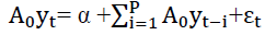 (1)
(1)
Where Yt is a (5*1) vector that contains (global crude oil production, global real economic activity, real oil prices, the KCFSI, the stock market returns A0 denote a contemporaneous coefficient matrix, α denotes a vector of constant terms, εt denote a vector of serially and mutually uncorrelated structural shocks, and p is the order of the SVAR which is set equal to two quarters according to the information criteria AIC, FPE. Under the appropriate identifying restrictions, the structural shocks can be recovered from the estimated reduced-form errors by using the following relationship:
 (2)
(2)
Where et denotes the reduced-form errors.
We then identified the Structural Vector Autoregressive (VAR) model by using the Choleski decomposition as well as the introduction of the variable order recommended by Kilian (2009). The criteria are the decreasing endogenous variables. This amounts to introducing the most exogenous to the top (the one that responds only to its own shock and is not sensitive to other variables) and the most endogenous variable in the end (the variable which is responsive to all the shocks affecting the system). Therefore, the selected order is then the world oil production, the index of the global economic activity, the WTI real oil price, the financial stress index KCFSI, and the stock returns.
According to Kilian (2009), global oil production is expected to be less sensitive probably due to the high adjustment costs of oil production, followed by the index of global oil demand. The last responds to the oil supply shocks almost immediately. According to Hamilton (1983) and Kilian (2009), the oil supply disruption has a significant influence on the global economic activity. The impact of the speculative oil demand can be explained by changes in the precautionary demand, which is included by the expected decline in the supply of oil and by uncertainty in future production. Therefore, it is plausible that this type of shock is placed third.
The index of the financial stress KCFSI, which enables to capture the financial shocks, is placed after the series of the real price of oil based on the assumption that oil prices have contemporary effects on financial markets, but not vice versa. This assumption is in line with that of Kilian and Park (2009), which employed a VAR model to investigating the response of the stock market fluctuations of the oil price shocks, with the ordering of the variables (oil supply, the real economic activity, the real oil prices, and the real stock returns). The last ones are classified according to the oil price shocks; because it is assumed that an impact on the price of oil will have an instant impact on the stock prices, while a shock to the share prices will not have an instant impact on the oil price shocks.
Hence, the reduced-form VAR is obtained by multiplying both sides of Eq. (1) by  This has the following recursive structure:
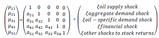 (3)
(3)
Thus, we can relate the shocks to the structural innovations as follows:
1. Oil supply shocks are innovations in oil supply.
2. Aggregate demand shocks are innovations in the global economic activity which cannot be explained by oil supply shocks.
3. Oil-specific shocks are innovations in crude oil prices which cannot be explained by the oil supply shocks or aggregate demand shocks.
4. Financial stocks are innovations for the global financial market conditions which cannot be explained by oil price shocks based on the assumption that oil prices have contemporaneous effects on the financial markets but not vice versa.
The other shocks to the stock returns are innovations in the stock prices which cannot be explained by four oil price shocks and the financial shocks above.
Results And Interpretation
We have estimated the relationship between structural shocks and stock market returns for equation (3). These estimation results are presented step by step as follows.
Unit Root Test
Most times series model and techniques require pre-testing the underlying series for unit root. For this reason, several attempts have been made to characterize the statistical properties. (Dickey and Fuller, 1981; Phillips and Perron, 1988; Elliott et al., 1996; Ng and Perron, 2001; Kwiatkowski et al., 1992).
Nevertheless, the conventional unit root test may be suspect since the analyzed sample contains major events ( the introduction of the Euro in 1999, the attack on the Twin Towers in New York on 11 September 2001, the global crisis of 2009), that are more likely to create structural breaks in the series. However, one may impose NP (2010) test which has been developed to test the unit root given the existence of structural breaks. Apart from this new unit root test, Narayan and Liu's (2015) work is the version that handles the possibility of heteroskedasticity in the series as well.
Evidently, different unit root test considered structural breaks over the period of time across the many areas of economics. A unit root test with known break dates (exogenous breaks) was intensified by innovations (Perron, 1989; Lee and Strazicich, 2013, Perron, 1997, Zivot and Andrews, 1992; Perron and Vogelsang, 1992). The list is far from being exhaustive. Another strand of research has examined a unit root test with likely estimated break dates (endogenous breaks). Important empirical studies include the following: Narayan and Popp (2010), Lee and Strazicich (2003), and Lumsdaine and Papell (1997) proceeded to consider two endogenous breaks. Further, Bai and Perron (2003) proposed multiple endogenous structural breaks on multiple time series data.
Following the tests above, this research has considered different possible unit root tests. In a first step, the stationarity of all variables is tested by a traditional unit root test of Dickey-Fuller (1997) without considering structural changes in the selected period of time, which has become widely popular over several decades. In a second step, this research has considered the Narayan and Popp's (2010) method in the presence of two endogenous structural breaks as an appropriate approach in this context. One of the studies which drew the attention to Narayan and Popp (2010) Test is by Nicolas and Keung (2015), Salisu et al., (2016). The empirical results for the two tests chosen are reported in the following Table 1A, Table 1B and Table 2.
| TABLE 1A ADF Test Of Global Stock Markets Returns |
|||||
| SMR-USA | SMR-Germany | SMR-France | SMR-Italy | SMR-Japan | |
| Level | |||||
| t-Statistic | -11.272 | -11.881 | -6.058 | -5.85 | -9.152 |
| Test critical value: 5% | -2.906* | -2.906* | -2.905* | -2.905* | -2.906* |
| First difference | -9.152 | -6.098 | -6.058 | -9.426 | -9.384 |
| Test critical value: 5% | -2.906* | -2.905* | -2.905* | -2.906* | -2.906* |
| TABLE 1B ADF Test Of Global Stock Markets Returns |
|||||
| SMR-Argentina | SMR-Brazil | SMR-Tunisia | SMR-Thailand | SMR-Jordan | |
| Level | |||||
| t-Statistic | -3.251 | -7.234 | -6.112 | -22.726 | -22.726 |
| Test critical value: 5% | -2.905* | -2.906* | -2.905* | -2.905* | -2.905* |
| First difference | -7.234 | -7.68 | -9.939 | -9.751 | -9.751 |
| Test critical value: 5% | -2.906* | -2.907* | -2.906* | -2.9092* | -2.9092* |
Note: The critical values of ADF test are lower than t-statistic: the variable is stationary. SMR designate, the stock market returns.
| TABLE 2 ADF Test Of Structural Oil Price Shocks And Financial Shocks |
||||
| Variables | ∆COP t | REA t | ROP t | KCFSI t |
| Level | ||||
| t-Statistic | -3.168 | -2.734 | -4.408 | -3.155 |
| Test critical values: 5% | -3.479 | -2.909 | -3.479* | -2.906* |
| First difference | -6.624 | -10.469 | -7.026 | -6.226 |
| Test critical values: 5% | -2.906* | -2.910* | -2.906* | -2.906* |
Note: The critical values of ADF test are lower than t-statistic: the variable is stationary.
The ADF test consists in checking the null hypothesis:
H0: (Non-stationarity) against the alternative hypothesis.
H1: (Stationarity) the decision is made by comparing the absolute value of the t-statistic to the critical value.
1. -If, critical value<t-statistic, we then accept the null hypothesis of non-stationarity of the variables considered.
2. -If, t-statistic<critical value, then, the null hypothesis of non-stationarity is rejected.
In order to study the stationary of the series of the structural model, we conducted unit root tests on all the series in level and in first differences. The ADF tests (Dickey and Fuller, 1981) have been used for this purpose to test the null hypothesis of non-stationary. The results in Tables 2 and 3 shows that the series of (COP, REA) are non-stationary in level with an absolute value of the t-statistics below the critical value. However, we note that the ADF value of the first difference reveals a statistically higher t-value in absolute value to the critical values for all series. These results lead to the acceptance of the null hypothesis of non-stationary for all the variables and we conclude that all variables are stationary on first difference.
However, the estimation of a SVAR model requires no co-integration between the sets. To this end, we conducted cointegration tests of Johanson (1988). The results found lead us to reject the existence of cointegration relationships between the structural shocks and the stock market returns in each country, which validates the application of the SVAR method in our study.
Table 3 presents the results of the Narayan and Popp (2010) unit root test. Regarding the variables (ΔCOP, REA, ROP and KCFSI), the null of the unit root for the majority variables could not be rejected only in the case of ROP using the quarterly frequency.
| TABLE 3 Narayan And Popp (2010) Unit Roots Test Results With Two Structural Breaks |
||||||
| M1 M2 | ||||||
| Break in intercept | Break in intercept and trend | |||||
| Country | Variables | |||||
| Test statistic | TB1 | TB2 | Test statistic | TB1 | TB2 | |
| Stationarity of structural oil price shocks and financial shocks | ||||||
| ∆COP | -1.243 | 2008 Q1 | 2007 Q4 | -6.375* | 2006 Q1 | 2006 Q1 |
| REA | -8.086* | 2002 Q4 | 2003 Q1 | -4.892** | 2002 Q2 | 2002 Q1 |
| ROP | -3.435 | 2013 Q1 | 2013 Q1 | -3.618 | 2012 Q1 | 2012 Q1 |
| KCFSI | -4.766** | 2004 Q4 | 2005 Q1 | -5.667* | 2011 Q4 | 2006 Q6 |
| Stationarity of global stock markets returns | ||||||
| SMR-USA | -6.842* | 2000 Q4 | 1999Q2 | -7.163* | 2000 Q4 | 1999 Q3 |
| SMR-Germany | -7.148* | 2002 Q3 | 2003Q2 | -7.056* | 2002 Q3 | 1999 Q3 |
| SMR-France | -6.848* | 2002 Q3 | 2009Q2 | -6.948* | 2002 Q3 | 1999 Q3 |
| SMR-Italy | -6.618* | 2008 Q4 | 2000Q1 | -6.4* | 2008 Q4 | 2000 Q1 |
| SMR-Japan | -7.009* | 2008 Q4 | 1999Q2 | -6.774* | 2008 Q4 | 2002 Q2 |
| SMR-Argentina | -6.16* | 2014 Q3 | 2009Q1 | -6.052* | 2014 Q2 | 2011 Q2 |
| SMR-Brazil | -6.912* | 2002 Q3 | 1999Q3 | -7.482* | 1999 Q2 | 1999 Q3 |
| SMR-Thailand | -28.67* | 2012 Q1 | 1999Q2 | -28.776* | 2012 Q1 | 1999 Q4 |
Note: TB1 and TB2 are the dates of the structural breaks.
M1 assuming both the breaks in intercept. Critical for M1= -4.949133, 4.443649, -4.193627 at 1%, 5%, 10%, respectively.
M2 assuming break in both intercept and trend. Critical values of M2=-5.347598, -4.859812, -4.607324 at 1%, 5%, 10%, respectively.
Overall, the results showed that COP, KCFSI and ROA display structural breaks at a 5% and 1% significance level. We also argue that the breaks-up dates occurred after the 9/11 attacks in 2001 and during subprime crisis that plaguing the economy since mid-2008, the impacts of which could very much still is seen in 2009, 2010, 2011 and 2012.
To give more details, it should be noted that the year 2008 marks a collapse in demand and violence in the movement of the oil price. During this year, prices continue to rise, peaking in excess of 145 & in July 2008, before dropping below 100& in October 2008. This drop in prices continues to reach values below 40 dollars in early 2009, resulting in structural breaks. However, according to data released by Federal Reserve Bank of Kansas City the KCFSI index reached high levels in the summer of 2007, a date that was often cited as the beginning of the subprime crisis.
To give more details, it should be noted that the year 2008 marks a collapse in global oil demand and oil price movements. During this year, the oil prices continued to increase until it peaks at about 145$ in July 2008. In the early 2009, downward pressure continued to impact oil prices, which reached 40$. These events have resulted structural breaks. However, according to the data released by the Federal Reserve Bank of Kansas City, the KCFSI index reached high levels in the summer of 2007, a date that was often cited as a structural break for the majority of the series.
Empirical evidence shows that the stock market returns are stationary with a two break at the 1% level. This means that the null of the unit root for the all series could not be rejected. As shown in Table 4, the break dates are different and quite close across countries
| TABLE 4 Variance Decomposition Of Developed Stock Market Returns |
|||||
| Variance decomposition of USA stock market returns | |||||
| Period | SMR_USA | COP | REA | ROP | KCFSI |
| 1 | 48.225 | 9.897 | 1 | 22.671 | 18.205 |
| 2 | 44.699 | 10.933 | 0.972 | 26.677 | 16.717 |
| 3 | 40.955 | 10.578 | 0.936 | 32.207 | 15.322 |
| 4 | 39.3 | 10.33 | 0.958 | 34.703 | 14.706 |
| 5 | 38.678 | 10.238 | 1.013 | 35.601 | 14.468 |
| 6 | 38.5 | 10.215 | 1.075 | 35.881 | 14.377 |
| 7 | 38.359 | 10.217 | 1.132 | 35.948 | 14.341 |
| 8 | 38.316 | 10.228 | 1.179 | 35.95 | 14.325 |
| 9 | 38.288 | 10.241 | 1.216 | 35.936 | 14.317 |
| 10 | 38.268 | 10.256 | 1.243 | 35.919 | 14.311 |
| Variance decomposition of Japan stock market returns | |||||
| Period | SMR_Japon | COP | REA | ROP | KCFSI |
| 1 | 69.438 | 0.265 | 0.016 | 0.023 | 30.254 |
| 2 | 62.310 | 0.944 | 1.681 | 8.509 | 26.552 |
| 3 | 54.439 | 1.626 | 3.641 | 13.349 | 26.943 |
| 4 | 50.789 | 2.027 | 5.141 | 14.866 | 27.173 |
| 5 | 49.327 | 2.275 | 6.185 | 15.169 | 27.041 |
| 6 | 48.709 | 2.453 | 6.865 | 15.146 | 26.824 |
| 7 | 48.389 | 2.602 | 7.283 | 15.072 | 26.652 |
| 8 | 48.176 | 2.745 | 7.530 | 15.007 | 26.539 |
| 9 | 48.012 | 2.892 | 7.673 | 14.956 | 26.465 |
| 10 | 47.873 | 3.051 | 7.754 | 14.912 | 26.409 |
| Variance decomposition of Germany stock market returns | |||||
| Period | SMR_Germany | COP | REA | ROP | KCFSI |
| 1 | 76.122 | 0.225 | 0.042 | 0.422 | 23.185 |
| 2 | 70.937 | 1.211 | 0.056 | 6.532 | 21.262 |
| 3 | 65.261 | 1.917 | 0.172 | 10.677 | 21.970 |
| 4 | 62.155 | 2.341 | 0.364 | 12.632 | 22.505 |
| 5 | 60.617 | 2.619 | 0.582 | 13.492 | 22.687 |
| 6 | 59.828 | 2.824 | 0.791 | 13.861 | 22.693 |
| 7 | 59.386 | 2.992 | 0.970 | 14.014 | 22.635 |
| 8 | 59.107 | 3.140 | 1.114 | 14.072 | 22.565 |
| 9 | 58.907 | 3.279 | 1.224 | 14.089 | 22.498 |
| 10 | 58.750 | 3.415 | 1.305 | 14.087 | 22.440 |
| Variance decomposition of France stock market returns | |||||
| Period | SMR_France | COP | REA | ROP | KCFSI |
| 1 | 76.409 | 1.643 | 0.129 | 0.0002 | 21.817 |
| 2 | 70.793 | 2.465 | 0.517 | 6.176 | 20.046 |
| 3 | 64.481 | 2.728 | 1.041 | 10.686 | 21.061 |
| 4 | 61.157 | 2.810 | 1.590 | 12.722 | 21.718 |
| 5 | 59.590 | 2.849 | 2.103 | 13.535 | 21.920 |
| 6 | 58.822 | 2.877 | 2.541 | 13.837 | 21.920 |
| 7 | 58.409 | 2.903 | 2.890 | 13.936 | 21.860 |
| 8 | 58.163 | 2.928 | 3.155 | 13.957 | 21.795 |
| 9 | 58.003 | 2.953 | 3.348 | 13.952 | 21.740 |
| 10 | 57.892 | 2.981 | 3.485 | 13.940 | 21.699 |
| Variance decomposition of Italy stock market returns | |||||
| Period | SMR_Italy | COP | REA | ROP | KCFSI |
| 1 | 73.341 | 4.631 | 0.458 | 0.263 | 21.305 |
| 2 | 65.309 | 5.398 | 1.362 | 7.950 | 19.979 |
| 3 | 57.562 | 5.220 | 2.294 | 13.393 | 21.528 |
| 4 | 53.924 | 5.045 | 3.159 | 15.606 | 22.264 |
| 5 | 52.336 | 4.962 | 3.920 | 16.383 | 22.397 |
| 6 | 51.580 | 4.928 | 4.548 | 16.621 | 22.321 |
| 7 | 51.164 | 4.918 | 5.038 | 16.669 | 22.208 |
| 8 | 50.904 | 4.921 | 5.407 | 16.657 | 22.109 |
| 9 | 50.728 | 4.931 | 5.675 | 16.629 | 22.034 |
| 10 | 50.601 | 4.949 | 5.867 | 16.601 | 21.979 |
Note: The results are based on the forecast error decomposition over the horizon of 12 month and units are in %.
SMR designate, the stock market returns
We first examine the results on the USA presented in Table 4 through a brief discussion of the critical values. The first break of this country took place in 1999; this regime change can be explained by the trend increase in the US trade deficit in 1999, which was reinforced by the Asian financial crisis. The second break date of 2000, which can also explained by the early 2000s recession that affected some developed countries such as the United States.
We next consider the results for Germany, France and Brazil. The findings indicate that in these countries, the null hypothesis of the unit root is rejected at a 1% significance level. The break point for these countries does exactly coincide with a serious recession of major events, such as, the recessions of the last decades, that which took place between 1990 and 1998, the first Gulf War in 1990-2014, the Asian financial crisis in 1997-1998, the Russian financial crisis in 1998, the global economic crisis in 2007 to 2012. Additionally, these events were characterized by a deregulation of the monetary system and a credit expansion.
Lastly, the structural break-up dates estimated for Argentina are generally different from those of other countries. As shown in the above table, the null of the unit root cannot be rejected in the presence of two structural breaks at a 1% significance level. The breaks in 2009-2014 provide apparent evidence for the impact on the evolution of public debt in Argentina on the economic growth.
Impulse Response to Structural Shocks
The response of the stock market returns by country of (supply shocks, aggregate demand shocks, oil-specific demand shocks, and financial shocks) is shown in Figures 1 and 2.
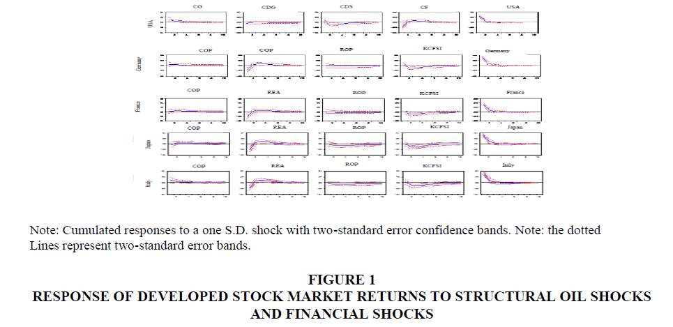
Figure 1: Response Of Developed Stock Market Returns To Structural Oil Shocks And Financial Shocks
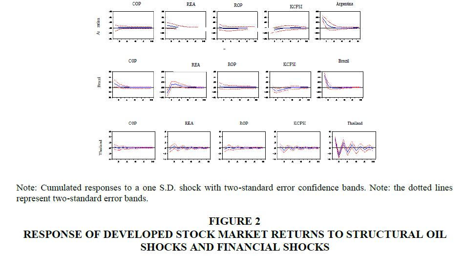
Figure 2: Response Of Developed Stock Market Returns To Structural Oil Shocks And Financial Shocks
Response of the stock market returns in the developed countries to the world oil price shocks
The first column in Figure 1 shows the responses of the stock market returns to the supply shocks in the developed countries. This does not cause a statistically significant impact on the stock returns in all the developed countries for a horizon of 10 quarters except the United States. This result is consistent with that of Cong et al., 2008, who concluded that oil supply shocks has no impact on the stock markets of India, Russia and China.
Moreover, the positive relation between an unexpected increase in the world oil production and the U.S stock market in the first quarter is explained by the lower production costs which motivate the increase of corporate profits, and therefore a permanent increase of the real stock market returns.
The second column shows that an unexpected increase of the world oil demand causes a statistically significant increase of the developed market returns except for the United States. We can see that in the first quarter, the effects of demand on the stock returns of Japan, France, Italy and Germany are negligible and not statistically significant. The world oil demand explains 1% of the variation of the stock market returns of 3 months. Over time, and in 8 quarters, the effect is greatly reduced and becomes insignificant. These results are consistent with the studies of Kilian and Park (2009), Apergis and Miller (2009) who also found that the global oil demand has a positive impact on the stock returns.
France and Germany have similar results. Each country seems to have generally stable dividend yields in response to the oil-specific demand shocks that persist for 10 quarters. However, an unexpected increase in the oil-specific demand shocks implies a persistent decline of the stock market returns in the three countries (Japan, Italy and USA).
This result leads us to conclude that this negative impact is likely to occur when the agents expect a lower global production due to political unrest in the oil producing countries, such as the Syrian civil war, the ongoing conflict in the Middle East during the period 2012-2013, the conflict in Iraq in 2003, the Nigerian conflict in 2005. All these events will create a positive impact of speculative demand, which increases the prices of oil, then causes a transfer of income from the net oil importing countries to the net oil exporting countries. This result is also consistent with several which studies show that increased speculation in the oil markets, due to the increased involvement of hedge funds and the financialization of the oil markets creates a strong correlation between oil prices and stock returns (Fattouh et al., 2013; Hamilton and Wu, 2012; Tang and Xiong, 2012; Alquist and Kilian, 2010; Buyuksahin et al., 2010; Silvennoinen and Thorp, 2010).
The impulse response of the stock returns to financial shocks is of particular interest in this article. An unexpected increase of the financial stress index KCFSI causes a statistically significant decrease of the stock returns in four developed countries (France, Italy, Germany and Japan). This result indicates that when the financial stress increases, financing costs become higher and more uncertainty depresses real economic activity, and therefore the market returns become lower. On the other hand, financial shocks cause a statistically significant increase of the stock returns in the United States. This positive relationship means that financial capital in the USA continues to circulate during the global financial stress. This result is not consistent with what was shown in the study of Chen et al. (2014) who found a positive financial impact causes a statistically significant decline of the stock market returns for France, Germany, Japan, and the United States. In the last column, analysis of the response functions shows that the stock markets react instantaneously and positively to its own shock. However, the effects of this shock fade after two quarters.
Response of stock returns in emerging countries to world oil prices shocks
The first column shows that a positive oil supply shock causes a statistically significant increase of the stock returns in Tunisia, Jordan and Brazil only in the first quarter. A plausible explanation is that the increase of the global oil supply reduces the oil prices and costs in the industry, and therefore increases the profit of the company. However, the results for other countries (Argentina and Thailand) may be attributed to the negligible impact of shocks to the supply of oil on the stock returns. This result is not consistent with the findings of Broadtock and Filis (2014).
According to the second column of Figure 2, we can say that the impact of the oil shocks driven by global oil demand on the stock returns in the emerging countries has been mixed. First, we found that only Brazil and Jordan have been affected by the aggregate demand shocks. This response reached its maximum after 3 quarters, and then started falling. This means that both stock markets of (Brazil and Jordan) reflect the positive ripple effect of the global economic expansion. Generally, when economic activity increases, the demand for oil increases and consequently the oil price increases. The results for Tunisia and Thailand show a less pronounced impact of the global demand reactions. This finding strengthens the relationship between the stock market and the oil price shocks, which should not be considered in a purely static environment. From this result, we can conclude that as long as oil prices do not because the oil consumption in these three countries, oil prices still has no significant impact on the economies. In these three countries, the limit of regulation and capital control are much more restricted than in other countries, since their stock markets are more distinct and independent from the global economy. Therefore, we can see that the impact of oil prices driven by global demand and speculative demand on the stock prices is less important.
A reading of the third column of Figure 2, shows that the impact of the oil-specific demand shock on the stock returns is insignificant for all the periods of 10 quarters, their reaction is negative. This suggests the idea that oil demand in these five countries should not be ranked in the precautionary demand due to uncertainty on supply deficits. This result is consistent with those of Degiannakis et al. (2013), who found that the oil-specific demand shocks have no significant impact on the stock returns of the European industrial sectors, which is not compatible with the study of Kilian and Park (2009), and Jung and Park (2009), who showed that the effect of the precautionary demand is highly significant.
In the last line, the unexpected increase of the financial shock causes a decrease of the stock returns in Jordan and Brazil. For this reason, the response of the stock returns to the financial shocks is not significantly over the period, except between the first and the sixth quarter. However, the reaction of the stock market returns of Tunisia and Argentina is significant only in the first quarter but not significant for the whole remaining period. In fact, as we have emphasized in column 4, the stock market returns in both emerging markets tend to move inversely to the financial shocks. Indeed, when the financial stress index undergoes a positive shock, the stock returns negatively react by a decline of the realized volatility.
The impulse response functions can be supplemented by an analysis of variance decomposition of the forecast error. The objective is to calculate the contribution of each of the innovations of the shocks of oil prices to the variance of the error of the stock market returns. In general, we write the variance of the forecast error at a horizon of one quarter (short term) to 10 quarters (long-term) according to the variance of the error assigned to each variable. The results relating to the variance of the decomposition of the study are reported in the following tables.
In line with the results of developed countries, the analysis of the response functions in the last column shows that the emerging stock markets (Argentina, Brazil, Tunisia, and Jordan) react instantaneously and positively to its own shock with a relatively short amortization period, approximately one quarter. However the effects of this shock are not significant for all remaining periods.
Variance Decomposition
To quantify the fraction of the stock market returns explained by the structural oil market shocks and underlying financial shocks. In fact, Tables 4 and 5 summarize the results of a forecast error variance decomposition of the real stock market returns for the ten countries in our sample.
| TABLE 5 Variance Decomposition Of Developed Stock Market Returns |
|||||
| Variance decomposition of Argentine stock market returns | |||||
| Period | SMR_Argentina | COP | REA | ROP | KCFSI |
| 1 | 87.617 | 0.067 | 0.775 | 11.477 | 0.062 |
| 2 | 85.103 | 0.121 | 0.757 | 13.964 | 0.053 |
| 3 | 83.832 | 0.254 | 1.072 | 14.781 | 0.057 |
| 4 | 83.331 | 0.388 | 1.338 | 14.878 | 0.062 |
| 5 | 83.114 | 0.505 | 1.474 | 14.840 | 0.065 |
| 6 | 82.963 | 0.611 | 1.521 | 14.837 | 0.065 |
| 7 | 82.825 | 0.714 | 1.531 | 14.862 | 0.065 |
| 8 | 82.697 | 0.823 | 1.530 | 14.882 | 0.066 |
| 9 | 82.578 | 0.940 | 1.527 | 14.884 | 0.068 |
| 10 | 82.465 | 1.069 | 1.525 | 14.867 | 0.071 |
| Variance decomposition of Brazil stock market returns | |||||
| Period | SMR_Brazil | COP | REA | ROP | KCFSI |
| 1 | 71.772 | 7.219 | 1.823 | 5.7120 | 13.472 |
| 2 | 63.991 | 7.517 | 1.688 | 15.063 | 11.738 |
| 3 | 58.940 | 7.097 | 1.564 | 21.348 | 11.048 |
| 4 | 57.347 | 6.903 | 1.526 | 23.310 | 10.911 |
| 5 | 56.959 | 6.847 | 1.528 | 23.754 | 10.908 |
| 6 | 56.875 | 6.837 | 1.544 | 23.819 | 10.922 |
| 7 | 56.850 | 6.837 | 1.564 | 23.816 | 10.930 |
| 8 | 56.832 | 6.840 | 1.584 | 23.809 | 10.933 |
| 9 | 56.816 | 6.843 | 1.601 | 23.804 | 10.933 |
| 10 | 56.801 | 6.847 | 1.616 | 23.800 | 10.933 |
| Variance decomposition of Jordan stock market returns | |||||
| Period | SMR_Jordan | COP | REA | ROP | KCFSI |
| 1 | 82.492 | 2.416 | 5.617 | 1.470 | 8.002 |
| 2 | 79.292 | 3.668 | 5.709 | 4.468 | 6.860 |
| 3 | 71.725 | 4.231 | 5.207 | 9.991 | 8.844 |
| 4 | 65.878 | 4.362 | 4.781 | 14.119 | 10.857 |
| 5 | 62.532 | 4.349 | 4.595 | 16.451 | 12.069 |
| 6 | 60.833 | 4.314 | 4.589 | 17.610 | 12.651 |
| 7 | 60.007 | 4.287 | 4.678 | 18.141 | 12.884 |
| 8 | 59.601 | 4.271 | 4.801 | 18.367 | 12.957 |
| 9 | 59.389 | 4.263 | 4.924 | 18.454 | 12.967 |
| 10 | 59.266 | 4.260 | 5.032 | 18.483 | 12.957 |
| Variance decomposition of Tunisia stock market returns | |||||
| Period | SMR_Tunisia | COP | REA | ROP | KCFSI |
| 1 | 85.122 | 4.0007 | 1.307 | 1.998 | 7.571 |
| 2 | 84.518 | 4.148 | 2.022 | 2.524 | 6.785 |
| 3 | 83.753 | 4.151 | 2.649 | 2.626 | 6.818 |
| 4 | 83.178 | 4.126 | 3.202 | 2.607 | 6.885 |
| 5 | 82.705 | 4.101 | 3.696 | 2.608 | 6.888 |
| 6 | 82.273 | 4.081 | 4.136 | 2.648 | 6.860 |
| 7 | 81.874 | 4.067 | 4.521 | 2.709 | 6.827 |
| 8 | 81.522 | 4.058 | 4.850 | 2.770 | 6.798 |
| 9 | 81.227 | 4.054 | 5.124 | 2.819 | 6.774 |
| 10 | 80.988 | 4.053 | 5.347 | 2.854 | 6.755 |
| Variance decomposition of Thailand stock market returns | |||||
| Period | SMR_Thailand | COP | REA | ROP | KCFSI |
| 1 | 91.562 | 1.184 | 1.311 | 3.726 | 2.214 |
| 2 | 88.103 | 0.768 | 1.266 | 5.760 | 4.100 |
| 3 | 88.370 | 0.845 | 1.273 | 5.604 | 3.905 |
| 4 | 88.050 | 0.768 | 1.275 | 5.800 | 4.104 |
| 5 | 88.025 | 0.806 | 1.267 | 5.808 | 4.092 |
| 6 | 87.990 | 0.779 | 1.277 | 5.834 | 4.118 |
| 7 | 87.946 | 0.805 | 1.268 | 5.848 | 4.130 |
| 8 | 87.942 | 0.796 | 1.277 | 5.853 | 4.130 |
| 9 | 87.914 | 0.817 | 1.271 | 5.857 | 4.138 |
| 10 | 87.908 | 0.816 | 1.277 | 5.861 | 4.136 |
Note: The results are based on the forecast error decomposition over the horizon of 12 month and units are in%.
SMR designate, the stock market returns.
The results in Table 4 show that the variance of the forecast error of the stock returns in the United States is due to 48.225% to its own innovations and 51.775 % of the change of the oil price shocks.
Contribution of the oil price shocks to variations of the stock market returns in the developed countries
In the short term, the variance of stock returns is caused by speculative demand shocks. This can be attributed to the presence of oil futures market. In the long term, the dominance of these shocks persists, but with a decrease of the share of the variance explained by the financial shock at 14.31%.
Based on the decomposition of the variance of Japan, Italy, Germany and France, the short and long term results of these four countries differ from those developed in the United States. In addition, the variance of the stock returns is explained by the impact of the speculative demand and the financial shocks at a rate of 35.63%. However, the shock in aggregate demand and of oil supply is not at the origin of the dominant part of the variance of the stock returns only in three countries (Italy, Germany, and France). By contrast, this relationship is particularly plausible in Japan since the world demand for oil shows a significant increase 7.75%, after 10 quarters than in the other three countries (Italy, Germany, and France) because of their strong economic growth. This relationship was illustrated by the impulse response functions (Figure 1).
When reading the results in Table 5, we note that the fluctuations of the stock returns of each emerging country are caused by its own shock with a very high proportion of 82.46% (Argentina), 56.80% (Brazil), 59.26% (Jordan), 80.98% (Tunisia), 87.90% (Thailand). By contrast, the share of the fluctuations of the stock returns realized by the innovations attributable to oil shocks is low.
These results show that the Tunisian stock market is very autonomous. However, the explanatory elements of the fluctuations of the stock market returns in Tunisia can occur only in the market, but not outside because of its weak integration into the global market. In the long term, all oil price shocks are an equal and a lower fraction representing about 19.009%. Despite its large opening and its small size, the Jordanian stock market is vulnerable to many exogenous shocks, including the impact of speculative demand and financial shocks which approximate 40.732% in the long term. However, the vulnerability of the Jordanian stock market to oil shocks has increased.
The contribution of the oil price shocks to variations of the stock market returns in the emerging countries
According to the result of Jordan, the variability of the stock returns for Brazil in the short and long term is driven by financial stocks followed by the shock of the speculative demand, while supply shocks and demand for oil represent only 8.46%.
Conclusion
This paper completes the literature existence in two sides. First, some literature established that the stock markets of the developed countries tend to react differently to different oil price shocks (Degiannakis et al., 2014; Basher et al., 2012; Kilian and Lewis, 2011; Kilian and Park, 2009; Apergis and Miller, 2009). However, the existing literature has not focused on the emerging countries. In this regard, we compare the effects of oil price shocks on the stock markets in the developed countries with those in the emerging countries using a structural VAR methodology proposed by Kilian and Park (2009). We found that the response of the emerging stock markets to oil price shocks is less important than the developed countries. A plausible explanation of this strength of the stock market of the developed countries to oil price shocks in the 1998-2014 period can be attributed to the fact that crude oil is of utmost importance for the developed countries than for the emerging ones. Overall, this result supports the hypothesis of departure.
The second major contribution to the existing literature is the study of the impact of financial shocks which is a determinant of the volatility of oil prices, according to the results derived from a study by Chen et al. (2014) on the stock returns. In this respect, we found that the unexpected increase of the index KCFSI implies an increase of the stress in the financial markets causing a decrease of the equity returns in the developed countries than in the emerging countries. This finding is consistent with the efficient market hypothesis of Basher et al. (2012), who assume that the efficient market can quickly respond to new information.
The results of this study offer several avenues of research. First, future research could be designed to evaluate how this relationship changes over time, through the application of the correlation models varying in time, such as the dynamic conditional correlation (DCC-GARCH).
Managerial Implications
First, the shocks caused by supply have generally a negligible impact on the stock returns, particularly for four developed countries (USA, France, Italy, Japan and Germany) but a positive impact on the stock returns of Tunisia, Jordan, Brazil and the USA only in the first quarter. This result due to the fact that disruptions in oil supply do not cause significant changes in oil prices, possibly because OPEC's decisions on oil supply levels are nowadays anticipated by all markets.
Second, oil price shocks caused by an unexpected increase of the world demand for all the industrial products lead to a persistent increase of real equity returns. This is very significant for four developed countries (Germany, Japan. France and Italy) and two emerging countries (Jordan, Brazil)). This means that the increase of oil demand is usually turned into significant economic gains, generating an increase in investment activity, consequently, a rise of the stock market returns of these six countries because of the existence of several sectors linked to consumption, such as distribution, luxury goods and automobile construction.
Thirdly, and as already highlighted in Graphs 1 and 2, a lower stock market returns in the developed countries such as (France, Germany, Japan and Italy) are likely to happen when oil prices are driven by a shock to a specific demand.
This can be attributed to the decreases in the global production because of international conflicts and political unrest in oil-producing countries, which will increase the oil spot prices in real terms and reduce the stock market returns. By cons, it is important to mention that, unlike in the developed countries, the relationship between the shock of speculative demand and stock returns is totally negligible. This implies that emerging markets are dominated by very active public enterprises on the market. Also, this result can be explained by the existence many effective strategies for oil hedging by corporations and emerging governments which absorbs the increases of oil price for their consumers.
References
- Abhyankar, A., Xu, B., & Wang, J. (2013). Oil price shocks and the stock market: Evidence from Japan. The Energy Journal, 34(2), 199-222.
- Alquist, R., & Kilian, L. (2010). What do we learn from the price of crude oil futures? Journal of Applied Econometrics, 25, 539-573.
- Apergis, N., & Miller, S.M. (2009). Do structural oil-market shocks affect stock prices? Energy Economics, 31, 569–575.
- Bai, J., & Perron, P. (2003). Computation and analysis of multiple structural change models. Journal of Applied Econometrics, 18(1), 1-22.
- Barsky, R., & Kilian, L. (2004). Oil and the macroeconomy since the 1970s. Journal of Economic Perspectives, 18(4), 115-134.
- Basak, S., & Pavlova, A. (2013). A model of financialization of commodities. The Journal of Finance, 71(4), 1511-1556.
- Basher, S.A., Haug, A.A., and Sadorsky, P. (2012). Oil prices, exchange rates and emerging stock markets. Energy Economics, 34, 227–240.
- Basher, S. A., & Sadorsky, P. (2006). Oil price risk and emerging stock markets. Global Finance Journal, 17, 224-251.
- Baumeister, C., & Peersman., G. (2012). The role of time-varying price elasticities in accounting for volatility changes in the crude oil market. Journal of Applied Econometrics, 28(7), 1087-1109.
- Broadstock, D.C., & Filis, G. (2014). Oil price shocks and stock market returns: New evidence from the United States and China. Journal of International Financial Markets, Institutions and Money, 33, 417-433.
- Buyuksahin, B., Haigh, M.S., & Robe, M.A. (2010). Commodities and equities: A market of one. Journal of Alternative Investments, 12(3), 76–95.
- Caporale, G.M., Menla Ali, F., & Spagnolo, N. (2015). Oil price uncertainty and sectoral stock returns in China A time-varying approach. China Economic Review, 34, 311-321.
- Chen, W., Hamori, S., & Kinkyo, T. (2014). Macroeconomic impacts of oil prices and underlying financial shocks. Journal of International Financial Markets, Institutions and Money, 9, 1–12.
- Cong, R.G., Wei, Y.M., Jiao, J.L., & Fan, Y. (2008). Relationships between oil price shocks and stock market: An empirical analysis from China. Energy Policy, 361(9), 3544–3567.
- Davig, T., & Hakkio, C. (2010). What is the effect of financial stress on economic activity? Federal Reserve Bank of Kansas City, Economic Review, 95(2), 35-62.
- Degiannakis, S., Filis, G., & Floros, C. (2013). Oil and stock returns: evidence from European industrial sector indices in a time-varying environment. Journal of International Financial Markets, Institutions and Money, 26, 175-191.
- Degiannakis, S., Filis, G., & Kizys, R. (2014). The effects of oil price shocks on stock market volatility: Evidence from European data. The Energy Journal, 35(1), 35–563.
- Dickey, D.A., & Fuller, W.A. (1981). Likelihood ratio statistics for autoregressive time series with a unit root. Econometrica. Econometria, 49(4), 1057-1072.
- Effiong, E.L. (2014). Oil price shocks and Nigeria stock market: What have we learned from crude oil market shocks? OPEC Energy Review, 38(1), 36-58.
- Elliott, G., Rothenberg, T.J., & Stock, J.H. (1996). Efficient tests for an autoregressive unit root. Econometrica, 64, 813–836.
- Fattouh, B., Kilian, L., & Mahadeva, L. (2013). The role of speculation in oil markets: what have we learned so far? Energy Journal, 34, 7–33.
- Filis, G., Degiannakis, S., & Floros, C. (2011). Dynamic correlation between stock market and oil prices: The case of oil-importing and oil-exporting countries. International Review of Financial Analysis, 20(3), 152-164.
- Gupta ,R., & Modise, M.P. (2013). Does the source of oil price shocks matter for South African stock returns? A structural VAR approach. Energy Economics, 40, 825-831.
- Hakkio, C.S., & Keeton, W.R. (2009). Financial stress: What is it, how can it be measured, and why does it matter? Federal Reserve Bank of Kansas City. Economic Review, 94(2), 5–50.
- Hamilton, J.D. (1983). Oil and the macroeconomy since World War II. Journal of Political Economy, 91, 228–248.
- Henderson, B.J., Pearson, N.D., & Wang, L. (2014). New evidence on the financialization of commodity markets. The Review of Financial Studies, 28(5), 1285-1311.
- Hamilton, J.D. (1996). This is what happened to the oil price–macroeconomy relationship. Journal of Monetary Economics, 38(2), 215-220.
- Hamilton, J.D., & Wu, J.C. (2012). Risk premia in crude oil futures prices. Journal of International Money and Finance, 42, 9-37.
- Hammoudeh, S., & Aleisa, E. (2004). Dynamic relationship among GCC stock markets and NYMEX oil futures. Contemporary Economic Policy, 22, 250-269.
- Hansol, J., & Cheolbeom, P. (2011). Stock market reaction to oil price shocks: A comparison between an oil-exporting economy and an oil-importing economy. Journal of Economic Theory and Econometrics, 22, 1–29.
- Henderson, B.J., Pearson, N.D., & Wang, L. (2014). New evidence on the financialization of commodity markets. The Review of Financial Studies, 28(5), 1285-1311.
- Hooker, M.A. (1996). What happened to the oil price-macroeconomy relationship? Journal of monetary Economics, 38(2), 195-213.
- Huntington, G.H. (2007). Oil shocks and real U.S. income. Energy Journal, 28(4), 31−46.
- Johanson, S. (1988). Statistical analysis of cointegrating vectors. Journal of Economic Dynamics and Control, 12, 231–254.
- Jones, D.W., Leiby, P.N., & Paik, I.K. (2004). Oil price shocks and the macroeconomy: What has been learned since 1996? Energy Journal, 25, 1–32.
- Jones, C.M., & Kaul, G. (1996). Oil and the stock markets. The journal of Finance, 51(2), 463-491.
- Jung, H., & Park, C. (2011). Stock market reaction to oil price shocks: a comparison between an oil-exporting economy and an oil-importing economy. Journal of Economic Theory and Econometrics, 22(3), 1–29.
- Kang, W., & Ratti, R.A. (2013). Oil shocks, policy uncertainty and stock market return. Journal of International Financial Markets, Institutions and Money, 26, 305– 318.
- Kilian, L. (2008). Exogenous oil supply shocks: How big are they and how much do they matter for the US economy? The Review of Economics and Statistics, 90(2), 216–240.
- Kilian, L., & Lewis, L.T. (2011). Does the Fed Respond to Oil Price Shocks? The Economic Journal 121(555), 1047-1072.
- Kilian, L. (2009). Not all oil price shocks are alike: disentangling demand and supply shocks in the crude oil market. American Economic Review, 99, 1053–1069.
- Kilian, L., & Park, C. (2009). The impact of oil price shocks on the U.S. stock market. International Economic Review, 50, 1267–1287.
- Kwiatkowski, D., Phillips, P.C., Schmidt, P., & Shin, Y. (1992). Testing the null hypothesis of stationarity against the alternative of a unit root: How sure are we that economic time series have a unit root? Journal of econometrics, 54(1-3), 159-178.
- Lee, J., & Strazicich, M.C. (2003). Minimum lagrange multiplier unit root test with two structural breaks. Review of economics and statistics, 85(4), 1082-1089.
- Lee, J., & Strazicich, M. (2013). Minimum LM unit root test with two structural break. Economics Bulletin, 33(4), 2483–2492.
- Lee, K., Ni, S., & Ratti, R. A. (1995). Oil shocks and the macroeconomy: The role of price variability. Energy Journal, 16(4), 39−56.
- Lescaroux, F., & Mignon, V. (2008). On the influence of oil prices on economic activity and other macroeconomic and financial variables CEPII. OPEC Energy Review, 32(4), 343-380.
- Lin, C.C., Fang, C.R., & Cheng, H.P. (2009). Relationships between oil price shocks and stock market: An empirical analysis from the greater China.
- Lippi, F., & Nobili, A. (2012). Oil and the macroeconomy: A quantitative structural analysis. Journal of the European Economic Association, 10(5), 1059-1083.
- Lumsdaine, R., & Papell, D. (1997). Multiple trend breaks and the unit root hypothesis. Review of economics and Statistics, 79(2), 212-218.
- Narayan, P.K., & Liu, R. (2015). A unit root model for trending time-series energy variables. Energy Economics, 50, 391-402.
- Narayan, P. K., & Popp, S. (2010). A new unit root test with two structural breaks in level and slope at unknown time. Journal of Applied Statistics, 37(9), 1425-1438.
- Nandha, M., & Faff, R. (2008). Does oil move equity prices? A global view. Energy Economics, 30(3), 986-997.
- Nazlioglu, S., Soytas, U., & Gupta, R. (2015). Oil prices and financial stress: A volatility spillover analysis. Energy Policy, 82, 278-288.
- Nicholas, A., & Keung, L.C. (2015). Structural breaks and electricity prices: Further evidence on the role of climate policy uncertainties in the Australian electricity market. Energy Economics, 52, 176-182.
- Ng, S., & Perron, P. (2001). Lag length selection and the construction of unit root tests with good size and power. Econometrica, 69(6), 1519-1554.
- Nissanke, M. (2012). Commodity market linkages in the global financial crisis: Excess volatility and development impacts. Journal of Development Studies, 48(6), 732–750.
- Morana, C. (2013). Oil price dynamics, macro-finance interactions and the role of financial speculations. Journal of Banking & Finance, 37(1), 206–226.
- Papapetrou, E. (2001). Oil price shocks, stock market, economic activity and employment in Greece. Energy Economics, 23(5), 511-532.
- Perron, P., & Vogelsang, T.J. (1992). Nonstationarity and level shifts with an application to purchasing power parity. Journal of Business & Economic Statistics, 10(3), 301-320.
- Perron, P. (1989). The great crash, the oil price shock and the unit root hypothesis. Econometrica, 57(6),1361-1401.
- Perron, P. (1997). Further evidence on breaking trend functions in macroeconomic variables. Journal of econometrics, 80(2), 355-385.
- Phillips, P.C.B., & Perron, P. (1988). Testing for unit roots in time series regression. Biometrika, 75(2), 599-607.
- Sadorsky, P. (1999). Oil price shocks and stock market activity. Energy economics, 21(5), 449-469.
- Salisu, A.A., Oloko, T.F., & Oyewole, O.J. (2016). Testing for martingale difference hypothesis with structural breaks: Evidence from Asiae Pacific foreign exchange markets. Borsa Istanbul Review, 16(4), 210-218.
- Silvennoinen, A., & Thorp, S. (2010). Financialization, crisis, and commodity correlation dynamics. Working Paper. Sydney, University of Technology.
- Tang, K., & Xiong, W. (2012). Index investing and the financialization of commodities. Financial Analysts Journal, 68, 54–74.
- Zivot, E., & Andrews, D. (1992). Further evidence on the great crash, the oil price shock, and the unit root hypothesis. Journal of Business Economics Statistics, 10, 251–270.