Keywords

Volatility, GARCH Family Model, Heteroskedasticity, Forecasting.

Abbreviations

ARCH: Autoregressive Conditional Heteroscedasticity

ARIMA: Autoregressive Integrated Moving Average

EGARCH: Exponential Generalized Autoregressive Conditional Heteroscedasticity

EHP: Environmental Health Programme

EHPEA: Ethiopian Horticulture Producer Exporters Association

EIA: Environmental Impact Assessment

EPRP: Export Led Poverty Reduction Programme

GARCH: Generalized Autoregressive Conditional Heteroscedasticity

GED: General Error Distribution.

ITC: International Trade Center

JETRO: Japan External Trade Organization

Background

Floriculture has become one of the important high value agricultural industries in many countries of the world (Singh et al., 2016). In the past, flowers were not of much economic importance. The science and art of commercial floriculture has been recognized as an economic activity with the potential for generating employment and earning valuable foreign exchange. The demand for flowers and ornamental plants for different needs like religious, official ceremonies, parties, house decoration, weddings, funerals, etc. is on the rise. This demand for fresh flowers and plants is increasing world-wide over the coming years (Sudhagar, 2013).

The Export Led Poverty Reduction Programme (EPRP) focused on direct interventions with ‘Least Developed Countries’ (LDCs) and developing countries that integrated poverty alleviation measures as a core element of national policies and trade strategies. The EPRP is designed to work at the community level to promote the establishment of export-oriented production activities (Ratnayake, 2016).

The flower industry is currently expanding all over the world. It created about 190000 employees throughout the developing world. Every year, about 30 billion dollar is generated from the International flower industry that cited by the (Workneh, 2007).

According to the report of the Export Promotion Department of Ministry of Trade and Industry (MoTI), flower export has generated 42.5 million USD. The export volume has increased from 1.6 million stems in 1999/2000 to 32 million stem in 2003/04. In value terms, the increase was from 382,346 USD in 1999/2000, to 2.9 million USD in 2002/2003, to 5.1 million USD in 2003/04 and 21.9 million USD in 2005/2006 (Workneh, 2007).

The low-cost cut flower exporting countries close to the equator, such as Kenya, Ethiopia, Ecuador, Colombia and Malaysia, have increased their global market share in cut flower trade. About 15 percent of total cut flower exports from Colombia were shipped by sea (Van Rijswick, 2015).

The floriculture sector is a relatively new established sector in Ethiopia and rapidly growing. Whereas only five farms were operative in 2002, there are more than 80 farms operating today on a total of 1,200 ha of land (Staelens et al., 2014).

The Ethiopian floriculture industry was started in the early 1990's. It created job opportunity for about 25,000 workers and when the total licensed floriculture development projects between July 1992 and July 2006 become operational, the total number of employees is expected to be 72,000 (Workneh, 2007).

Due to the seasonal demand of flower trade, with peak demands at certain moments (for example Valentine’s day, Mother’s day and Easter) and low demand during northern summer, the sector has the reputation of hiring workers on an insecure basis (Riisgaard, 2011).

This study will be conducting on recent developments of floriculture industry in Bahirdar, Ethiopia, particularly in terms of sales of stem flowers and the growth of the industry and its trade with the world. The primary focus is on the export sales of flowers time series modeling.

Methods

Data for the Study

The study was conducted at Bahirdar Tanaflora PLC, Tanaflora private limited company was established on 14th February 2008 by Gafat Endowment and Threma-Fin Flora with each having 50% shares. This study employed secondary data obtain from Tana flora for the time of 2012-2017 production years of 72 consecutive months. Export sales of flower stems are recorded on monthly basis.

Data Analysis

Time series analysis often requires one to turn a non-stationary series into a stationary one so as to use this theory (Peter & Brockwell, 1996). We must transform non-stationary data to stationary data before moving forward with an evaluation. There are different methods of checking stationarity time series. Some of time plot and unit root test are ADF and PP unit root test. In this study a univariate Box-Jenkins Methods (Box & Pierce, 1970) and volatility models such as ARCH, GARCH, EGARCH and TGARCH models were conducted for forecasting export sales of flower. The majority of the work on time series analysis has been highly concentrated on univariate models, which are the simplest types to work with. Within this area, most work has been concentrated on the family of linear models, which includes the autoregressive (AR), moving average (MA) and autoregressive moving average models (ARMA) (Box & Pierce, 1970), and nonlinear models like ARCH, GARCH, EGARCH and TGARCH. In the Volatility, Heteroskedasticity affects the accuracy of forecast confidence limits and thus has to be handled properly by constructing appropriate non-constant variance models (Bollerslev, 1986; Taylor, 1994) independently generalized Engle's model to make it more realistic; the generalization was called “GARCH”. So far the modeling of the time series considered has assumed time invariant or constant variance. However in real life variance may change with time (a phenomenon defined as Heteroskedasticity), hence there is a need for models that accommodate this possible variation in variance (Bollerslev, 1986; Taylor, 1994). This is done by relating the error variance to the previous errors in the case of ARCH. In the case of GARCH, the previous conditional variances are included. The ARCH-GARCH modeling considers the conditional error variance as a function of the past realization of the series.

Results

The data considered in this paper were the monthly export sales of flower of 72 observationfrom January 2012-December 2017. The monthly average export sales of Tana flora was $405733.30 USD and the maximum export was $2956179 USD. In general the trend of the monthly export sales of flower tends to increase with some seasonality (Details can be found in Figure 1 & 2).

The seasonal component removed from the original data; the resulting values are called the “seasonally adjusted” data. If the variation due to seasonality is not of primary interest, the seasonally adjusted series can be useful. The time plot in Figure 2 shows that the export sales of flower do not follow a specific symmetric trend. It is also clear that there is no form of seasonality nor periodicity but only upward and downward moving trend in the export sales of Flower. That is an irregular swinging pattern in the data.

The result of the stationarity of the original sales of flower series at level form (Table 1), from a result of ADF and PP unit root test of the series shows that the t-statistics greater than the critical values 1%, 5% and 10% levels of significance respectively so we do not reject the null hypothesis. Therefore, the series do not satisfy the stationary assumption at level form with intercept and trend and intercept value. The first difference of the original sales of flower series changes in to stationary data (Details can be found in Figure 3). In the normality of the series, the null hypothesis for the Jarque-Bera test is the observations are normal while rejecting the null indicates the distribution of the data is non-Gaussian (not normal). From the Figure 4 Jarque- Bera test indicates that the first order differenced export sales of flower series is not normally distributed because we have evidence reject the null hypothesis.

Table 1 Test of stationary Adf and pp test for the export sales of flower (at level form)
Series	Include test equation	Test statistic		Test critical value
Flower		ADF	PP	1% level	5% level	10% level	Prob.
	With intercept	2.223665	0.506026	-3.528515	-2.904198	-2.589562	0.9999
	with trend and intercept	1.126618	-1.038162	-4.096614	-3.47627	-3.165610	0.9999

From the result of Tables 2 & 3, In the Portmanteau test, the null hypothesis is that the variable follows a white noise process and just like in any other statistical inference, a p-value that is smaller than the significance level, α (the probability of rejecting a true null hypothesis, usually set at α = 0.05) means that we reject the null and conclude that the variable is not a white noise.

Table 2 White noise test Portmanteau test for white noise
Portmanteau (Q) statistic	666.0404
Prob>chi2(34)	0.0000

 

Table 3 Arch- Lm Test For Integrated Model I (1) With Conditional Variance
F-statistic	33.26330	Prob. F(1,68)	0.0000
Obs*R-squared	22.99383	Prob. Chi-Square(1)	0.0000

ARCH-LM test is performed on the residuals of serial linear regression, and the test object of the F statistic is the joint significance of the squared residuals of all lags. The Obs*R2 statistic is the LM test statistic, which is the number of observations T multiplied by the test regression R2. Given the significance level α=0.05 and the degree of freedom 1, the value of LM is 22.99383 greater than the critical value of 3.841, and the concomitant probability P is 0.0000, which is less than 0.05. The null hypothesis is rejected. It shows that there is obvious Heteroskedasticity in the return sequence, and the residual has strong ARCH effect. Therefore, it is reasonable for this article to use the GARCH model to simulate the export sales of flower we can see in Table 4.

Table 4 Model Selection Criteria For The Symmetric Garch Models Arch (1) With Garch (1, 1) Under Distributions
Model	Distribution	AIC	BIC
ARCH(1)	T-distribution	27.33331	27.49266
	General error	27.34431	27.50366
GARCH (1, 1)	T-distribution	27.29312	27.48433
	General error	27.16779	27.39087

The non- linear time series models were deal to the monthly export sales of flower series. In the export sales of flower data, the best GARCH family model was known on the basis of in sample of the data.

The appropriate symmetric or asymmetric GARCH models can be selected using the information criteria. The models having smaller AIC or BIC are selected (we can found table 5). The output of Table 5 indicates that the symmetric GARCH model is selected based on AIC and BIC criteria. However, the estimated coefficient values do not satisfy the non-negativity α>0,β>0 the stability condition α₁+β₁ not less than one knowing the symmetric GARCH is not appropriated models to fit our research (the export sale of flora) data, we have to assess the appropriate and best non-linear asymmetric GARCH families. The Persistence determines to show how rapidly the variance forecast converges to the unconditional variance. In this study we compare to the symmetric GARCH models and asymmetric GARCH families of TGARCH and EGARCH models using conditional stability (we can found Table 6).

Table 5 The Conditional Stability Convergence of Garch and Asymmetric Model
Model	Positivity	Leverage effect	Asymmetric Impact	Stationarity
GARCH	-	-	-
TGARCH	Always
EGARCH	Always

 

Table 6 Comparison of Asymmetric Garch Family of, Egarch And Tgarch With Distributions and Their Conditional Stability
Model	Distribution	Coefficients			Cond. stability	Inf. Criteria
		α	β	γ		AIC	BIC
GARCH(1, 1)	T-distribution	0.459	0.712	-	Not	27.4843	27.369
	General error	1.5764	-0.128	-	Not	27.16779	27.3908
EGARCH (1, 1)	T-distribution	1.0957	0.802	-0.524	Yes	27.12554	27.3804
	General error	0.3899	-0.237	0.389	Yes	27.39663	27.61971
TGARCH(1, 1)	T-distribution	0.2912	0.726	0.564	No	27.28264	27.50572
	General error	0.2693	0.737	0.658	No	27.27822	27.50130

These models are important in estimating and forecasting volatility, as well as in capturing asymmetry, which is the different effects on conditional volatility of positive and negative effects of equal magnitude, and supposedly in capturing leverage. The leverage effect stems from the fact that losses have a greater influence on future volatilities than do gains. Asymmetry means that the distribution of losses has a heavier tail than the distribution of gains. Information criteria and statistical tests of the significance of the symmetry and leverage parameters are used to compare the models (we can found Table 7).

Table 7 Model Selection Criteria For The Candidate Egarch Models Under Distributions
Model	Distribution	AIC	BIC	Cond. stability
EGARCH (1,1)	T-distribution	27.12554	27.38049	Yes
	General error	27.39663	27.61971	Yes
EGARCH (1,2)	T-distribution	27.18648	27.44143	Yes
	General error	26.98147	27.26829	Yes
EGARCH(2,1)	T-distribution	27.40445	27.65940	Yes
	General error	27.42707	27.68202	Yes
EGARCH(2,2)	T-distribution	27.14259	27.42941	Yes
	General error	27.30572	27.59254	Yes

In model selection process, in order to achieve parsimonious model that captures and also most applications used the minimum order of GARCH models. First fit different GARCH family models the orders of p=1 and q=1. We employ in the GARCH family models GARCH (1,1), EGARCH (1,1) and TGARCH (1,1) under the distribution of t- distribution and GED. To select the best fit model used different statistical such selection criteria, the minimum value of the information criteria (AIC, BIC), according to coefficient value (stability, the asymmetric impact and leverage effects).

From Table 7, we understand the best-fit model is selected from the asymmetric GARCH models that EGARCH (1,1) model under t-distribution has fulfills the stability condition, asymmetric impact and leverage effect in (we can found Table 6). Furthermore, within the asymmetric, in EGARCH model used different orders p=1,2 and q=1,2 compare EGARCH (1,1), EGARCH (1,2), EGARCH (2,1) and EGARCH (2,2) models, the minimum information criteria and also the others is considered to be EGARCH (1,2) under the general error distribution (GED) better fit for modeling the conditional volatility of Tana flora monthly export sales of flower the research data (Table 8).

Estimating of Export Sales of Flower using EGARCH (1, 2) Model under GED

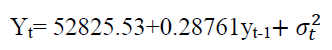
Now, we estimated the EGARCH (1,2) model, the maximum likelihood estimator that used. The model selected by the help of the minimum information criteria (AIC, BIC) within this the estimated model provides the parameter coefficient values for conditional variance equation . The conditional variance equation gives hence, the EGARCH (1,2) model can be written into conditional mean and conditional variance equations are:

The values of conditional standard deviation are obtained by taking the square root from the conditional variances. The plot from Figure 5 have there is up and down spikes indicates high volatile periods of the series. In the EGARCH (1,2) model, the volatile clustering will be detected.

Diagnostic Checking of EGARCH (1, 2)

In this part, we assessed how well the selected EGARCH (1,2) model, the Ljung-Box Q-test for the squared residuals are used and the presence of ARCH effects test ARCH-LM test. To do this we have used diagnostic checking for independence of the squared residuals (Table 9) and whether the presence or not of ARCH effect. From the result of Table 8 the correlogram squared residuals of the model show the insignificant p-value greater than 0.05. Hence, we have enough evidence to conclude that there is no autocorrelation in the squared residual of export sales of flower. The EGARCH (1,2) model is adequate to specify the conditional volatility equation and the standardized squared residuals fulfilled the identically independent condition.

Table 8 Correlogram Squared Residuals of Egarch (1, 2) Model
Lag	Q-statistics	Prob.
1	0.5752	0.448
2	2.9365	0.23
3	3.0039	0.391
4	5.8105	0.214
5	7.8508	0.165

 

Table 9 Arch-Lm Test For Egarch (1, 2) Model
F-statistic	1.502106	Prob. F(2,66)	0.2302
Obs*R-squared	3.004029	Prob. Chi-Square(2)	0.2227

Discussion

This study was to model the export sales of Tana flora for the period of January 2012- December 2017 production years of 72 consecutive months. Export sales of flower stems are recorded on monthly basis. The paper employed different univariate specifications of the Generalized Autoregressive Conditional Heteroscedastic (GARCH) model, including both symmetric and asymmetric models. The prediction of a future value used forecasting performance accuracy.

From the test of ARCH effect existence of the volatility of the data flower exports using monthly data this finding consistence with the flower export performance of Uganda study by (Okot & Nyanzi, 2014).

The export performance of sales of flower is showing a remarkable for the last six years. However, the unit prices of stem show the existence of fluctuation from period to period but in the previous study the unit prices of stem show a decline from period to period within the five years. Evaluation of Financial and operating performance of floriculture firms in Ethiopia (Doctoral dissertation, Addis Ababa University).

In literature most of the studies consistence report a study conducted (Mohiuddin, 2016) flower prices at the Dutch flower auctions were extremely volatile. Modeling of the volatility of data the Garch family in financial data.

The empirical results suggest that EGARCH model fits the sample data better than GARCH model in modeling the volatility of the series (Chiu et al., 2018).

In the Fluctuation period (crisis period), asymmetric GARCH model is preferred than symmetric GARCH, asymmetric models are the better models used to represent the stock market volatility during the economic fluctuation periods asymmetric GARCH model(s) can be the better model in capturing volatility of stock market (Lim & Sek, 2013).

Conclusion

This study examined the export sales of flower volatility on Tanaflora monthly data from the period of January 2012- December 2017. In measuring price volatility of the Tanaflora in Ethiopia against the U.S. dollar, this study employed the GARCH family volatility models.

The empirical results suggest that EGARCH model fits the sample data better than GARCH model in modeling the volatility of the series export sales of stem flower.

These models are important in estimating and forecasting volatility, as well as in capturing asymmetry nonlinear models in export sales of flower. Based on the minimum value of accuracy measures, the estimated model that is good enough to describe the data set is EGARCH (1,2) model with distribution of GED. Therefore, the minimum value of forecasting accuracy measure for MAPE is 52.37 and Theil’s is 0.16 which is an indication of good forecasting models. The forecasted results obtained from EGARCH (1,2) model shows that the export sales of flower are maturated and declining from January 2018-December 2019 with some fluctuations (volatility).

Declarations

Ethics Approval and Consent to Participate: Not Applicable

Consent to publication: This manuscript has not been published elsewhere and is not under consideration in any other journal.

Availability of data and materials: The data used in this study can be obtained on the secondary data from Tanaflora industry.

Competing Interests: The authors declare that they have no conflict of interests.

Funding: No fund was obtained for the study.

Authors’ Contributions: TKW and SA conceived the study, TKW analyzed the data, TKW and SA interpreted the results and drafted the manuscript. TKW finalized the manuscript to the present form. All authors have read and approved the manuscript.

Acknowledgement

The authors acknowledge the Tanaflora industry Bahirdar for providing the data.

References

Bollerslev, T. (1986). Generalized autoregressive conditional Heteroskedasticity. Journal of Econometrics, 31(3), 307-327.

Indexed at, Google Scholar, Cross Ref

Box, G.E.P., & Pierce, D.A. (1970). Distribution of residual autocorrelations in autoregressive-integrated moving average time series models. Journal of the American statistical Association, 65(332), 1509-1526.

Indexed at, Google Scholar, Cross Ref

Chiu, C.J., Harris, R.D.F., Stoja, E., & Chin, M. (2018). Financial market volatility, macroeconomic fundamentals and investor sentiment. Journal of Banking & Finance, 92, 130-145.

Indexed at, Google Scholar, Cross Ref

Lim, C.M., & Sek, S.K. (2013). Comparing the performances of GARCH-type models in capturing the stock market volatility in Malaysia. Procedia Economics and Finance, 5, 478-487.

Indexed at, Google Scholar, Cross Ref

Mohiuddin, M.D. (2016). Flower business flourishes floriculture: A study on Bangladesh. International Journal of Business and Management Invention, 5(10), 09-13.

Google Scholar

Okot, N., & Nyanzi, S. (2014). Bank of Uganda.

Indexed at, Google Scholar

Peter, J., & Brockwell, R.A.D. (1996). Introduction to time series and forecasting.

Indexed at, Google Scholar

Ratnayake, I. (2016). The experiences of New Zealand floriculture export producers in the changing international market: what can be done to strengthen the sector's capabilities.

Indexed at, Google Scholar

Riisgaard, L. (2011). Towards more stringent sustainability standards? Trends in the cut flower industry. Review of African Political Economy, 38(129), 435-453.

Indexed at, Google Scholar, Cross Ref

Singh, B.K., Rakesh, E.S., Yadav., V.P.S., & Singh, D.K. (2016). Adoption of commercial cut flower production technology in Meerut. Indian Research Journal of Extension Education, 10(1), 50-53.

Google Scholar

Staelens, L., Louche, C., & Haese, M.D. (2014). Understanding job satisfaction in a labor intensive sector: Empirical evidence from the Ethiopian cut flower industry. Paper presented at the presentation at the EAAE 2014 Congress. Agri-food and rural innovations for healthier societies.

Google Scholar

Sudhagar, S. (2013). Production and marketing of cut flower (Rose and Gerbera) in Hosur taluk. International Journal of Business and Management Invention, 2(5), 15-25.

Google Scholar

Taylor, S.J. (1994). Modeling stochastic volatility: A review and comparative study. Mathematical Finance, 4(2), 183-204.

Indexed at, Google Scholar, Cross Ref

Van Rijswick, C. (2015). World floriculture map 2015. Rabobank Industry Note.

Google Scholar

Workneh, T. (2007). An assessment of the working condition of flower farm workers: A case study of four flower farms in Oromia Region.

Received: 03-Apr-2022, Manuscript No. JEEER-22-11674; Editor assigned: 05-Apr-2022, PreQC No. JEEER-22-11674(PQ); Reviewed: 19-Apr-2022, QC No. JEEER-22-11674; Published: 26-Apr-2022