Keywords

Two Warehouse Inventory Model, Perishable Products, Product Life Cycle.

Introduction

In most of the studies it is assumed that the organization owns a single warehouse with infinite capacity. Although it is impossible for organizations to have a warehouse to manage the complete at particular time, therefore in practice, whenever a large stock is to be held, due to the limited capacity of owned warehouse (OW), one additional warehouse is taken on lease or rent. In certain practical situations, when suppliers provide price discounts for bulk purchases or when the item under consideration is a seasonal product such as the output of harvest or the replenishment cost is higher than the other related cost, etc., or the new product launched considering the large demand, the inventory manager may purchase more goods that can be stored in its own warehouse (OW) as this is a temporary phenomenon, therefore considering economical point of view, the distributors usually choose to rent other warehouses than rebuild a new warehouse. Thus, the excess quantity is stored in a rented warehouse (RW). The inventory costs (including holding cost and deterioration cost) in RW are usually higher than those in OW due to additional cost of maintenance, material handling etc. To reduce the inventory costs, it will be economical to consume the goods of RW at the earliest. Consequently, the firm stores goods in OW before RW, but clears the stocks in RW before OW. Therefore, the stocks of OW will not be released until the stocks of RW are exhausted (Goswami & Chaudhari, 1992; Benkherouf, 1997).

Literature Review

Hartley (1976) was the first to consider the effect of two warehouses. Sarma (1987) has considered the phenomenon of deterioration in two warehouses. Yang et al. (2004) proposed a two-warehouse model for deteriorating items with constant demand rate under inflation. Dye et al. (2007) proposed a two-warehouse model for deteriorating items with capacity constraint and time proportional backlogging rate. Tsao & Sheen, (2008) considered the case of dynamic pricing, promotion and replenishment for a perishable item subject to the supplier's trade credit and retailer's promotional effort. Roy & Choudhari, (2009) also worked on two production inventory models for deteriorating items when the demand rate depends on the instantaneous inventory level. Shah & Shukla (2009) has developed an inventory model in which product is subject to constant deterioration and shortages are allowed. Jie et al. (2010) had formulated a lotsizing model for deteriorating goods with a current-stock-dependent demand and delay in payments. Mahata (2012) had investigated the optimal retailer’s replenishment decisions for deteriorating items under two levels of trade credit policy to reflect supply chain management within the economic production quantity (EPQ) framework. Liao et al. (2013) had designed recently a two-warehouse inventory model for deteriorating items when the supplier offers the retailer a delay period and in turn the retailer provides a delay period to their customers. Dash et al. (2014) developed an inventory model for perishable goods with exponential decreasing demand and time dependent holding cost.

Ata & Nematolla, (2014) formulated a model for deteriorating items with back-ordering and financial considerations. Jaggi et al. (2017) worked on inventory model for deteriorating items with imperfect quality under the conditions of permissible delay in payment Singh (2017) obtained an optimal ordering policy for deteriorating items having constant demand.

In this study a two-warehouse model for items having very short life cycle is considered, initially demand increase exponentially and become constant after some time and finally decreases exponentially, the time value of money and inflation are also considered. This model is unique in itself as it is first time that all these factors are considered together, this model is well suited for electronic items and technology driven products. In this study, therefore I have considered opportunity cost and company will try to reduce opportunity cost to its minimum. Numerical solution of the model also supports the validity of the model (Pakkala & Achary, 1992).

Assumptions and Notations

The following assumptions and Notations are used in this paper

Assumptions

1. The product considered here has a very short life span

2. Initially demand increases exponentially for initial phase, become constant after

3. certain time and then start decreasing exponentially.

4. The time horizon of the inventory system is finite

5. Replenishment rate is infinite

6. Lead time is zero

7. The goods of OW are consumed only after consuming the goods kept in RW

8. Holding cost in RW warehouse is more than that is in OW

Notations and Symbols used in the model

i Inventory carrying rate.

A Ordering cost of inventory, Rupees/order.

T Length of inventory cycle, time unit

De^λt Exponential demand rate

θ₁ Rate of deterioration per unit time for RW

θ₂ Rate of deterioration per unit time for OW

W The capacity of owned ware house

t_w The time at which inventory level reaches zero in RW

I₁ (t) The level of positive inventory in RW at time t

I₂ (t) The level of positive inventory in OW at time t

c The purchasing cost

p The selling price per unit, where p>c

O Opportunity cost

Methodology

Considering the above assumptions, the inventory is depleted not only by demand but also by deterioration. Therefore, differential equation model has been developed. During the interval (0, t_w), the inventory levels are positive at RW and OW considering exponentially increasing demand. At RW, the inventory is depleted by the combined effect of demand and deterioration, while at OW inventory is depleted only by the effect of deterioration as to save on holding cost the organization would be first consuming the goods of the rented warehouse. Hence, the inventory level at RW and OW are governed by the following differential equation

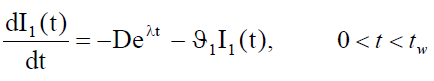(1)

with the boundary condition I₁ (t_w) = 0 and

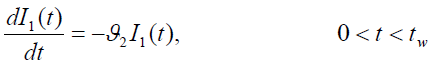(2)

with the initial condition I (0) =W 2 , respectively. Solving the differential equation (1) and (2) respectively, we get the inventory level as follows:

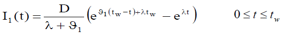(3)

(4)

During the interval (t_w, t₁), the inventory in OW is depleted due to combined effects of demand and deterioration. Hence, the inventory level at OW is governed by the following differential equation

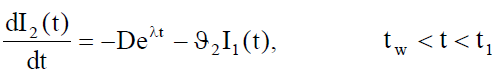(5)

with boundary condition I₂ (t₁) = 0. Solving the above equation, we obtain the inventory level as

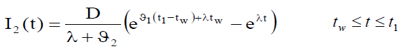(6)

Due to continuity at I₂ (t) at point t = t_w, it follows from equations (4) and (6), then

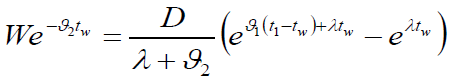(7)

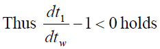
which implies that

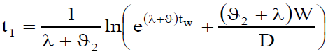(8)

The above equation gives t₁ in terms of t_w, hence

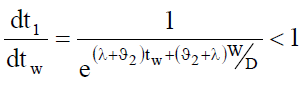(9)

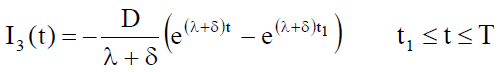
(10)

with the boundary condition I₃ (t₁) = 0

(11)

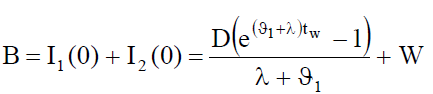
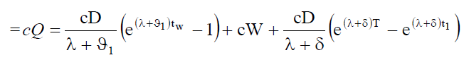
Therefore, requisite ordering quantity is

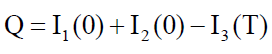
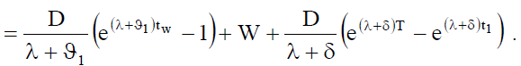(12)

(13)

For inflation rate f, the continuous time inflation factor for the time period t is given by e^ft which means that an item which costs $c at t = 0 will cost ce^ft at time t. Also, we have discount rate, r, representing the time value of money, thus we have present value factor for the time period t, is e^-rt. Therefore, the net inflation factor is ce^ft e^-rt. Thus, for an item with initial price Rupees c per unit, the present value of the inflated price of an item at time t =0, c0 is given by

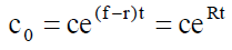(14)

In this cost c is inflated by the net inflation factor R. Thus, R is the present value of the inflation rate similarly, the present value of the inflated backorder cost c_b, c^b₀ is given by

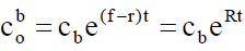(15)

Ordering cost is $ A/ order

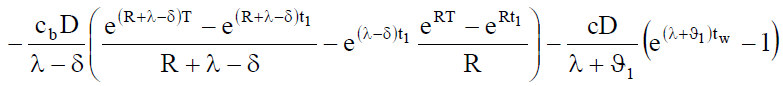
Holding cost per cycle in Rented Warehouse under inflation is given by

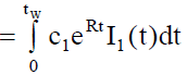
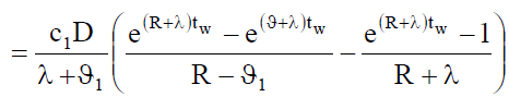(16)

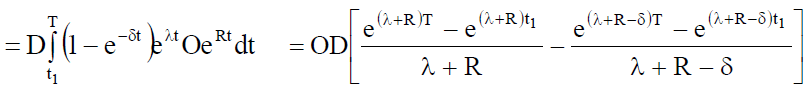
Holding cost per cycle in Own Warehouse under inflation is given by

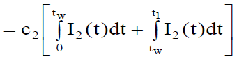
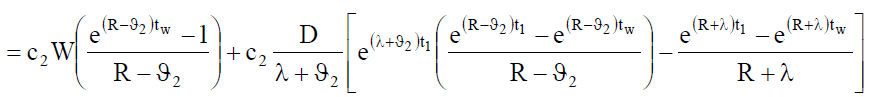(17)

Shortage cost per cycle under inflation is given by unmet demand during period (t1, T)

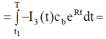
(18)

Opportunity cost due to lost sales per cycle under inflation is given by

(19)

As purchasing is done in the starting of cycle, therefore it is not affected by the effect inflation

Purchase cost per cycle is given

(20)

Sales revenue per cycle is given by

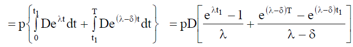(21)

Profit per cycle is given by Sales Revenue – Total Cost

Sales Revenue-Ordering Cost –Holding Cost-shortage Cost-Opportunity Cost-Purchase Cost i.e.

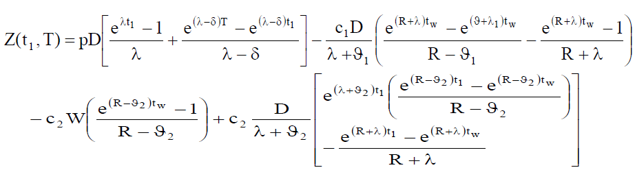
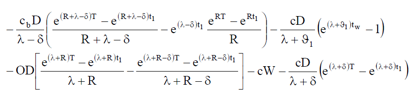(22)

Multiple Inventories Cycles per Year

As we have many cycles in a year and since inflation and time value of money exit during each cycle, hence we have to consider their effect over the time horizon, NT. Let there be N complete cycles during a year. Therefore, NT=1. The total profit during a year is given by

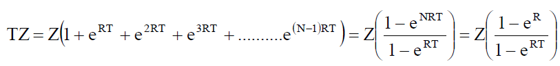(23)

As life cycle of the product has shrunk after certain time t, the demand after time t is constant, if demand D is more than the capacity of the Owned warehouse than only rented warehouse, we have to substitute λ = 0 i.e. demand is constant and the remaining calculations would remain same. In the case D is not more than the capacity of the owned warehouse, there is no need for the rented warehouse. Hence it is converted into the inventory model with constant demand and deterioration rate.

Similarly, in the third phase of the life cycle demand decreases exponentially we have to replace λ with negative β and again follow the same process. This case exists only when D is more than the capacity of the OW.

Observations & Results

Considering a practical case of a product having shrunk life cycle and considering the values of the parameters. Exponential parameter λ = .20, we obtained t₁ = 3weeks, if f=.07, r= 2 percent, Ordering cost =$10, D=1000 units, W=100 units, c₁ = 4.5, c₂ = 1.5.

TZ= $330, where =10 t_w days i.e. the rented warehouse is required only for 10 days each cycle of 1.5 months.

Conclusion and Future Orientations

In this paper problem of two warehouses has been considered for items having shrunk life cycle, initially exponentially increasing demand and constant rate of deterioration followed by constant demand and exponentially decreasing demand. The stock of RW warehouse is used first and stock of OW is used only after the stock in RW reaches zero. This is first time twowarehouse problem is considered for items having exponentially increasing demand. As it is not possible to store large stock of items for exponentially increasing demand. In this study holding cost for RW is more than OW, thus organization will try to finish the stock of RW warehouse first then OW.

This study is helpful in deciding optimal replenishment rate for items having exponential increasing demand for shorter span with different rate of deterioration for RW and OW. In this study we considered opportunity cost also, so that organization tries to reduce shortages so that they can serve customer to their full satisfaction. The proposed model can be extended in numerous ways. For example, we may extend the model considering only two phases of product life cycle or four phases of product life cycle. Also, we could extend the model to incorporate some realistic features, such as quantity discount or the unit purchase cost, the inventory holding cost, and others are also fluctuating with time.

References

1. Ata, A.T., & Nematolla, M. (2014). An inventory control problem for deteriorating items with back-ordering and financial considerations. Applied Mathematical Modelling, 38(1) 93-109.
2. Benkherouf, L. (1997). A deterministic order level inventory model for deteriorating items with two storage facilities. International Journal of Production Economics, 48(2), 167-175.
3. Dash, B.P., Singh, T., & Pattnayak, H. (2014). An Inventory Model for Deteriorating Items with Exponential Declining Demand and Time-Varying Holding Cost. American Journal of Operations Research, 4, 1-7.
4. Dye, C.Y., Ouyang, L.Y., & Hsieh, T.P. (2007). Deterministic inventory model for deteriorating items with capacity constraints and time proportional backlogging rate. European Journal of Operation Research, 178, 789-807.
5. Goswami, A., & Chaudhari, K.S. (1992). An economic order quantity model for items with two levels of storage for a linear trend in demand. Journal of the Operational Research Society, 43(2), 157-167.
6. Hartley, R.V. (1976). A Managerial Emphasis.  Good Year Publishing Company, California, Operations Research, 315-17.
7. Jaggi, C.K., Cardenas, L.E., Barron, S., Tiwari, & Shafi, A.A. (2017). Two warehouse inventory model for deteriorating items with imperfect quality under the conditions of permissible delay in payment. Scientia Iranica E, 24(1), 390-412. http://scientiairanica.sharif.edu/article_4042.html
8. Jie, M.Z., Yong, W., & Zhap, J. (2010). An inventory model for deteriorating items under stock-dependent demand and two-level trade credit. Applied Mathematical Modelling, 34(11), 2010, 3273-3285.
9. Liao, J.J., Chung, K.J., & Huang, K.N. (2013). A deterministic inventory model for deteriorating items with two warehouses and trade credit in a supply chain system. International Journal of Production Economics, 146(2), 557-565. https://ideas.repec.org/a/eee/proeco/v146y2013i2p557-565.html
10. Mahata, G.C. (2012). An EPQ inventory model for exponentially deteriorating items under retail partial trade policy in supply chain, Experts Systems with Application, 39(3), 3537-3550. DOI: 10.1016/j.eswa.2011.09.044
11. Pakkala, T.P.M., & Achary, K.K. (1992). Discrete time inventory model for deteriorating items with two warehouses. Opsearch, 29, 90-103. https://doi.org/10.1016/0377-2217(92)90306-T
12. Roy, T., & Chaudhari, K.S., (2009). A production inventory model under stock-dependent demand, Weibull distribution deterioration and shortage. International Federation Operational Research Society, 16(3), 325-346. https://doi.org/10.1111/j.1475-3995.2008.00676.x
13. Sarma, K.V.S. (1987). A deterministic order level inventory model for deteriorating items with two storage facilities. European Journal of Operation Research, 29(1), 70-73. https://doi.org/10.1016/0377-2217(87)90194-9
14. Shah, N.H., & Shukla, K.T. (2009). Deteriorating Inventory Model for waiting time Partial Backlogging. Applied Mathematical Sciences, 3(9), 421-428.  Corpus ID: 15957284.
15. Singh, S. (2017). Optimal ordering policy for deteriorating items having constant demand and deterioration rate. Theoretical Economics Letters, 7, 2152-2158.  https://www.scirp.org/pdf/tel_2017121115044058.pdf
16. Tsao, Y.C., & Sheen, G.J. (2008). Dynamic pricing, promotion and replenishment policies for a deteriorating item under permissible delay in payments. Computers and Operations Research, 35(11), 3562-3580.
17. Yang, H.L., Teng, J.T., & Chern, M.S. (2004). Two-warehouse inventory models for deteriorating items with shortages under inflation. European Journal of Operational Research, 157(2), 344-356.