Research Article: 2018 Vol: 19 Issue: 4
When does the stem gender gap emerge? Evidence from science fairs
Nanneh Chehras, University of California, Irvine
Abstract
Keywords
STEM, Gender Gaps, Science Fair.
Introduction
For decades, the gender gap in Science, Technology, Engineering, and Mathematics (STEM) fields has caused concern among policymakers and researchers (Sweeney, 1953; Fennema & Sherman, 1977; Goldin, 1994; Hausmann, 2009). Growing worry has prompted calls for the U.S. education system to produce more female graduates with training and expertise in STEM fields (Toulmin & Groome, 2007; Olson & Riordan, 2012). Yet, while female enrollment in high school math and science courses increases, and female performance on math tests improves, female participation in the STEM labor force has remained constant at 24 percent since 2000 (Beede et al., 2011).
Policymakers use the lack of progress in reducing the STEM gender gap to motivate a shift toward targeting K-12 students (Venkataraman et al., 2010). However, disagreement on when the STEM gender gap emerges makes developing effective policy difficult (Subrahmanyan & Bozonie 1996; Blickenstaff, 2005). The lack of agreement is due to shortcomings in conventional gender gap measures including standardized test scores, classroom performance, and classroom enrollment. Standardized test scores produce mixed results, depending on the year, age group, and exam (Ellison & Swanson, 2010). More importantly, exams do not measure, nor do they claim to measure, a student’s desire to pursue a STEM occupation (Popham, 1999). Classroom enrollment options are limited and generally only available to high school juniors and seniors, reducing the ability to capture gender differentials across STEM fields or among younger students (Hill et al., 2010). Further, college admission requirements incentivize students to perform well on exams and in classrooms (Clinedinst & Koranteng, 2014), reducing the ability to identify college major plans based on performance. Collectively, these measures fail to explain the timing of the STEM gender gap.
In this paper, a novel STEM gender gap measure to document the age profile of gender differentials has created. To do so, a dataset of high school and middle school science fair projects at the California State Science Fair (CSSF) has constructed and students’ project choices to measure gender gaps used.
This gender gap measure has three advantages. First, the CSSF allows for a wide range of projects, allowing the study of gender gap emergence age for a variety of fields. Second, with over 17,000 participants between 1990 and 2014 and approximately 60 percent middle school representation, studied students earlier in their academic careers. Third, the category in which a student competes is determined by his or her choice of project and although the incentive to perform well for college admissions still exists, it is less clear why it would drive the field of study. Thus, compared to conventional gender gap measures, CSSF participation is an improved measure of a student’s STEM engagement.
The analysis produces two main findings. First, it is to find significant gender gaps in middle school. For example, middle school females are 29 percentage points less likely to compete in a math field and 35 percentage points less likely to compete in a technology field, relative to social science. Second, gender gaps generally increase from middle school to high school. High school females are 37 percentage points and 42 percentage points less likely to compete in math and technology, respectively.
This paper’s findings have two policy implications. First, large gender differentials among middle school students suggest that efforts to reduce the STEM gender gap may be best targeted during elementary school or earlier. Second, policymakers should consider the widening of the gap from middle school to high school to prevent females from dropping out of the STEM pipeline. They types of policy programs vary in practice, but may take the form of introducing girls to STEM role models, breaking down STEM stereotypes, or communicating the relevance of STEM degrees to real-world applications. Wang & Degol (2017) offer evidence-based recommendations for policy and practice to improve STEM diversity.
Previous Findings On The Emergence Of The Stem Gender Gap
The STEM gender gap literature draws from two primary sources of information on high school and middle school performance: standardized test scores and classroom outcomes. This study presents the overall findings of each and discusses shortcomings to support the use of science fair projects as an alternative and improved source of information.
Test Score Findings
Between the two gender gap measures, standardized test scores are more commonly studied. The National Assessment of Educational Progress (NAEP), a nationally representative sample, is the primary resource supported by the U.S. Department of Education. Perie et al. (2005) provide a long-term assessment of gender differences for students ages nine, 13, and 17. Until the late 1980s, nine year old females score slightly higher on the mathematics exam. Among 13 year olds, males start to outperform females in the early 1980s, while males in the oldest age group consistently score higher since 1973. In 2004, the gender gap is significant only for students ages 13 and 17, suggesting that gender gaps in test scores emerges toward the end of middle school. Two additional exams include the Scholastic Aptitude Test (SAT) and American College Testing (ACT) exams. Males outperform females on the quantitative section of the SAT continuously since 1972, on average. Similar results hold for the quantitative section of the ACT, however, both SAT and ACT average differences are small in magnitude (Halpern et al., 2007).
Hyde et al. (1990) perform a meta-analysis of 100 studies and find that the math gender gap for the general population is trivial. Further analysis shows a female advantage in computation in elementary and middle school, and no gender differences in understanding of concepts at any age. Relatively large gender differences favoring males in complex problem solving skills emerge in high school. Hyde et al. (2008) conclude that the general population no longer shows differences in math skills, challenging the previously discussed findings using the NAEP data.
Researchers often compare U.S. test scores to international data to motivate a discussion about how social differences affect the emergence and evolution of gender gaps. Although social influence is outside the scope of this paper, the two most common sources, the Program for International Student Assessment (PISA) and the Trends in International Mathematics and Science Study (TIMSS), reveal patterns consistent with the findings that gender differences do not exist. For example, Lemke et al. (2001) find insignificant gender differences in TIMSS scores in the United States. Lindberg et al. (2010) perform a meta-analysis of the 2003 TIMSS and the PISA, representing 493,495 students, and find that all of the mean mathematics effect sizes are very small.
Classroom Findings
The second gender gap information source, classroom outcomes, describes how males and females differ in classroom subject choices and their performance in those classes. Since 1994, high school girls earn more maths and science credits and achieves higher grades. For example, among U.S. high school students, 66 percent of females compared to 58 percent of males enroll in chemistry, 93 percent of females compared to 89 percent of males enroll in biology, and 71 percent of females compared to 65 percent of males enroll in Algebra II. However, larger shares of male students take Calculus (12 percent of males compared to 11 percent of females) and physics (34 percent of males compared to 29 percent of females). Advanced Placement (AP) and Honors course enrollment data also shows an overrepresentation of females in math classes (54 percent) and science classes (56 percent), however, males are more likely to take the AP exam and score four percent higher on AP Calculus exams and six percent higher on AP science exams (Freeman, 2004).
Current Gender Gap Measure Issues
Standardized test scores, classroom performance, and classroom enrollment measures of the gender gap are limited in their abilities to capture student interest, which is correlated with future occupation. In this paper, STEM interest is defined as the desire to learn more about the field potentially resulting in a STEM career, or be engaged in the field beyond classroom requirements. Studies that establish the important role of interest include Tai et al. (2006). They use the National Education Longitudinal Study of 1988, where eighth-grade students are asked about the career they desire at age 30, and find that students who report science interest are three times more likely to obtain a college degree in a science field. The study does not discuss differences by gender. Maltese & Tai (2010) interview 116 scientists and graduate students in chemistry and physics and find that over 65 percent of male and female participants report interest starting before middle school. The purpose of the study is to establish that interest in science plays a role in future occupations, not to discuss gender differentials.
Although new test score estimates garner considerable attention, most findings produce relatively small gender differences. Thus, exams provide little practical importance in learning about when the gender gap emerges (Ellison & Swanson, 2010). Further, Weinberger (2005) shows that less than one-third of college-educated white males in STEM occupations have high school SAT quantitative scores above 650 (out of 800). She concludes that gender differentials in the workforce cannot be explained by standardized test differentials. Others make similar statements and explain that exams are designed to measure student knowledge, no interest. A recent National Research Council (2011) report states that although difficult, it is critical to measure student interest and motivation, creativity, or commitment and “not just good test takers.”
Incentivizes to perform well for college admission boards complicate the ability to measure gender gaps in interest using test scores, classroom enrollment, and grades. The National Association for College Admission Counseling (NACAC) lists grades, particularly in difficult classes, and standardized admission tests among the top factors in admission decisions. Thus, enrollment in higher level quantitative courses and performance may be a better indicator of the desire to go to college, rather than interest in a particular field.
Classroom enrollment statistics of gender gaps are further complicated by state graduation requirements. For example, during the time period studied in the paper, students in California generally follow the “traditional pathway” which consists of Algebra I, Geometry, Algebra II, Pre-calculus, AP Calculus or AP Statistics. Students in California must complete at least two math courses in high school, with one or a combination of courses meeting or exceeding Algebra I rigor (California Department of Education, 2014). Students are often encouraged to follow a predetermined series of classes, which restricts the ability to measure student interest in a subject. Additionally, subject choices are often reserved for older students and are limited in the number of options. For example, among the 2013 high school graduating class, 88 percent of AP biology exams are taken in 11th or 12th grades. AP Calculus had 98.5 percent and AP Chemistry had 93.3 percent of students take the exam in their last two years of high school.
Science Fair Advantages
By the above test score measures, gender gaps in the general population do not exist today, while classroom enrollment suggests that they may emerge in 11th and 12th grades, leading policymakers to perhaps erroneously conclude that gender gaps do not exist prior to the end of high school. CSSF project choice is an improved source of gender gap information because it is not subject to the limitations outlined above. First, the category in which a student competes in is determined by a student’s choice of project, reflecting interest in a STEM field. The CSSF explicitly states that one of its objectives is to stimulate interest and recognize students for their efforts. A potential concern is that the choice of project is also motivated by a desire to get into college. For example, students may choose to participate in more difficult categories strictly to improve their college admission prospects, not because they are interested in the topic. Although the incentive to perform well for college admission boards exists at the CSSF, it is less clear that student project type would be influenced, especially compared to advanced courses, which are explicitly favored by admission boards.
In order to participate in the CSSF, students must receive an offer from their regional fair. Most regional fairs are structured similarly to the CSSF in that students are interviewed by several judges to showcase their knowledge, genuine interest, and enthusiasm for their work. Thus, a CSSF project is an improved measure of student interest. Second, as discussed in the next section, the large sample of middle school students at the CSSF allows for the study of younger students. Finally, with a large range of categories to compete in, measured gender differentials in each STEM field, category, and compare those values to existing measures.
Data
Construct the CSSF dataset using publicly available individual-specific information from 1990 through 2014. Each year has information for every CSSF participant, including name, grade, division, category, school, and county. This timeframe produces a well-powered sample to detect conservative overall and subject-specific gender gaps.
Participant gender is not explicitly stated. To determine gender, data from a 100 percent sample of Social Security card applications for U.S. births are used. In a given year, the Social Security Administration (SSA) records the number of males and females born with a name and reports frequency counts of those names by sex, as long as the name is at least two characters long with a frequency of at least five. The student’s grade and year of participation are used to estimate his or her birth year. Then match the student’s first name to the SSA data in his or her birth year to determine gender (Assume that participants’ current names represent the gender they identify with). If a name applies to both males and females, assign the majority gender as long as at least 90 percent of children born with that name have the same gender. This method assigns gender to 86 percent of participants. The paper’s results are robust to alternative cutoffs of 85 and 95 percent. The less conservative cutoff of 85 percent increases the sample by 124 students and the 95 percent cutoff decreases the sample by 466 students.
Assign gender to half of the remaining 2,651 participants using individual portraits which become available in 2005. Approximately 51 percent of the gender entries identified through photos are female. The paper’s results are robust to excluding these individuals. In total, there are 17,265 participants with identified gender.
Middle school students in grades six through eight compete in the Junior Division, while high school students in grades nine through 12 compete in the Senior Division. The number of Junior Division participants generally increases over the 25 year period (Figure 1). Senior Division participation exhibits an increase in earlier years, declines in the late 1990s, and remains relatively stable after with an average of 245 students per year. There are always fewer Senior Division participants in each year.
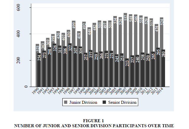
Figure 1: Number Of Junior And Senior Division Participants Over Time
Within division, students are further divided into categories based on their projects. The number of categories grows over time. In 1990, there are 13 Senior Division Categories and 13 Junior Division categories. By 2014, there are 14 categories for Senior Division projects and 22 categories for Junior Division projects. Categories are renamed, combined, or divided in response to changes in participation. The CSSF descriptions of yearly changes are used to make categories constant over time, when applicable. For example, in 2002, the CSSF renames biochemistry to biochemistry/molecular biology and combing the both categories under the second title. Figure 2 displays number of participants by category.
Using the Economics and Statistics Administration’s STEM definitions, the group categories labeled into the four STEM fields. For example, biology is labeled “science,” while environmental engineering is labeled “engineering.” The majority of students compete in a STEM category, with the highest concentration in science, followed by engineering. Math and technology fields are the least popular (Table 1 and Figure 2). Appendix 1 lists the categories with brief descriptions.
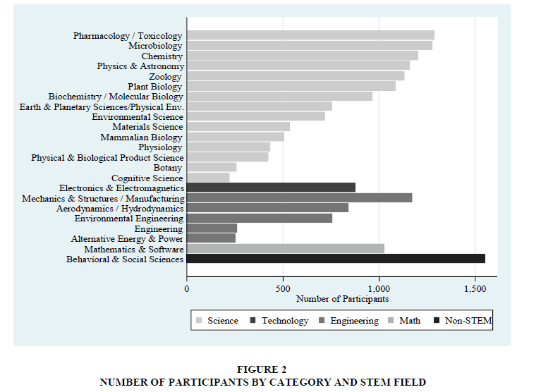
Figure 2: Number Of Participants By Category And Stem Field
| Table 1 Sample Composition |
||
| Junior Division | Senior Division | |
| STEM | 91% | 92% |
| Science | 63% | 65% |
| Technology | 5% | 5% |
| Engineering | 19% | 14% |
| Math | 4% | 8% |
| N Participants | 11,133 | 6,132 |
Methodology
In the following section, female participation trends are shown in Figure 3. Gender gap patterns are clear through the figure; however, to estimate significance and the significance of changes across age the following specification is used:
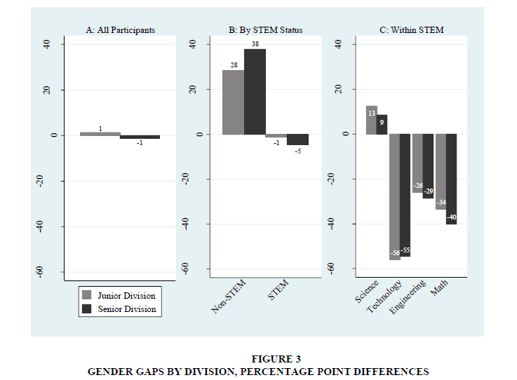
Figure 3: Gender Gaps By Division, Percentage Point Differences
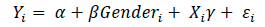 (1)
(1)
Where, Genderiis an indicator that equals one if student is female. The magnitude of β for Junior and Senior Division participants is interested if changes across age are significant. Yi represents several outcome variables. The first is an indicator that equals one if the student competes in a STEM field and zero otherwise. Second, create outcome variables to compare each STEM field against non-STEM categories. Third, create three indicators comparing technology, engineering, or mathematics against science. Largely driven by biology and chemistry, science exhibits the most balanced gender composition and is thus used as the comparison group to study within STEM variation.
CSSF participants represent counties throughout California. To account for time-invariant gender norm differences across California on the relative number of females in STEM Xi includes student country. Include county dummies as students are chosen at the county-level to proceed to the state competition. Sufficient variation within schools or districts does not exist to include indicators are lower levels. Xi also includes year dummies.
There are three sources of bias that challenge the claim that CSSF gender gaps reflect differences in interests. The first two are created by the qualification process, which dictates that CSSF participants are students who participate, win, receive a CSSF offer, and accept a CSSF offer at their local county science fairs. First, bias due to gender-specific student self-selection potentially exists at two levels: county fair participation and CSSF offer acceptance. Second, bias due to gender-specific selection by judges exists at the remaining qualification levels: county fair winners and CSSF offers. The third source of bias is due to changing yearly samples of students.
Gender-specific student self-selection at the county level, if relevant, results in CSSF gender gap estimates that are biased downward. Niederle’s (2014) summary paper finds that after controlling for a variety of characteristics, gender gaps in tournament entry in stereotypical male tasks persist. Additionally, Niederle & Yestrumskas (2008) find that, conditional on performance, females shy away from difficult and challenging tasks more than males.
Although field experiments produce less conclusive results compared to lab experiments, if gender-specific reactions to competing in male-dominated fields holds in this setting, then the gender gaps observed at county are underestimates. If county science fair participation becomes part of the school curriculum, for example, then the females, who would otherwise not compete, would likely enter in less male-dominated fields, increasing the gender gap.
Gender-specific student self-selection from county to state, however, would result in overestimates of gender gaps. If females are more likely to decline an offer to the CSSF, especially if they would have to compete in male-dominated fields, then this paper’s findings are biased upward.
The direction of bias due to gender-specific selection by judges is unclear. Consider the two extreme cases. In scenario one, there are no gender gaps at the county-level, but large gaps at the CSSF, while the opposite holds in scenario two. Thus, CSSF gender gaps are a result of who wins and who is selected to receive an offer, reflecting differences in factors other than interests, like performance or judge discrimination.
Finally, the long time period may mask underlying trends about the evolution of gender gaps over time. For example, any gender gaps observed with the pooled data may be driven by results in the earlier time period producing misleading conclusions. Further, any observed gender gap changes during this time period may be due to changes in the underlying mechanisms that determine gender gaps or due to changing samples.
In order to ease estimation concerns due to the qualification process, to construct a county-level dataset and evaluate gender gaps at lower levels. Repeated the above regression analysis and discuss findings below. To evaluate if gender gaps change over time, estimate β by five-year intervals. Five-year intervals has chosen to overcome small sample sizes in the year-to-year samples and test the null hypothesis that βt is equal to βt-1. Additionally, interact Genderi with Year and test for a non-zero time-trend. Interpretation in the context of changing samples is discussed below.
Science Fair Gender Gaps
Female participation patterns are displayed in Figure 3. A value of zero indicates balanced gender composition. Negative values indicate an underrepresentation of females and bar heights correspond to the percentage point difference between female and male participation. Among all CSSF participants, male and female participation is balanced, with differences less than two percentage points (Figure 3, Panel A). Figure 3, Panel B further divides students by whether they compete in a STEM category. STEM fields are generally balanced, while non-STEM fields are dominated by females. There is also large increase in female representation from the Junior to Senior Divisions in non-STEM. Further separating participants by each STEM field produces large gender differentials within STEM (Figure 3, Panel C). Technology, engineering, and mathematics are dominated by male participants, and the gender differentials become larger from Junior to Senior Divisions. For example, the largest gender differentials are in the technology fields with 55 and 57 percentage point gaps in the Junior and Senior Divisions, respectively. Science fields have more female than male participants; however, the magnitude of gender gaps is smaller than the gender gaps in other STEM fields that favor males.
Table 2 shows the regression results for all participants, while Tables 3 & 4 separate by division. Each table displays the results with and without the county and year dummies. Table 2 includes all outcome variables. Outcome variables using non-STEM as the comparison group are found in Table 3, while within STEM results, which use science as the comparison group, are found in Table 4. Finally, Tables 3 & 4, Column 5 display the absolute value of t-statistics, testing the hypothesis that βJunior = βSenior.
| Table 2 Gender Gap Regression Results |
||||
| Dep Var | STEM vs. Non-STEM | Science vs. Non-STEM | ||
| Gender | -0.052*** | -0.053*** | -0.042*** | -0.044*** |
| (0.004) | (0.004) | (0.006) | (0.006) | |
| County | x | x | ||
| Year | x | x | ||
| N | 17265 | 17265 | 12463 | 12463 |
| Dep Var | Technology vs. Non-STEM | Technology vs. Science | ||
| Gender | -0.400*** | -0.382*** | -0.085*** | -0.084*** |
| (0.018) | (0.018) | (0.005) | (0.005) | |
| County | x | x | ||
| Year | x | x | ||
| N | 2250 | 2250 | 11831 | 11831 |
| Dep Var | Engineering vs. Non-STEM | Engineering vs. Science | ||
| Gender | -0.255*** | -0.250*** | -0.129*** | -0.127*** |
| (0.013) | (0.013) | (0.007) | (0.007) | |
| County | x | x | ||
| Year | x | x | ||
| N | 4509 | 4509 | 14090 | 14090 |
| Dep Var | Math vs. Non-STEM | Math vs. Science | ||
| Gender | -0.326*** | -0.312*** | -0.069*** | -0.066*** |
| (0.019) | (0.019) | (0.005) | (0.005) | |
| County | x | x | ||
| Year | x | x | ||
| N | 2366 | 2366 | 11947 | 11947 |
| Note: ***p<0.001. | ||||
| Gender is a dummy variable that equals one if the participant is female. | ||||
| Table 3 Gender Gaps By Division |
|||||
| Junior Division | Senior Division | Junior Division | Senior Division | T-Statistic | |
| (1) | (2) | (3) | (4) | (5) | |
| Dep Var: STEM vs. Non-STEM | |||||
| Gender | -0.046*** | -0.062*** | -0.048*** | -0.062*** | 1.538 |
| (0.005) | (0.007) | (0.005) | (0.007) | ||
| County & Year Dummies | x | x | |||
| N | 11133 | 6132 | 11133 | 6132 | |
| Dep Var: Science vs. Non-STEM | |||||
| Gender | -0.033*** | -0.058*** | -0.037*** | -0.059*** | 1.699 |
| (0.007) | (0.009) | (0.007) | (0.009) | ||
| County & Year Dummies | x | x | |||
| N | 7996 | 4467 | 7996 | 4467 | |
| Dep Var: Technology vs. Non-STEM | |||||
| Gender | -0.380*** | -0.439*** | -0.355*** | -0.417*** | 1.546 |
| (0.023) | (0.031) | (0.023) | (0.032) | ||
| County & Year Dummies | x | x | |||
| N | 1459 | 791 | 1459 | 791 | |
| Dep Var: Engineering vs. Non-STEM | |||||
| Gender | -0.232*** | -0.304*** | -0.224*** | -0.304*** | 2.449 |
| (0.016) | (0.024) | (0.016) | (0.024) | ||
| County & Year Dummies | x | x | |||
| N | 3124 | 1385 | 3124 | 1385 | |
| Dep Var: Math vs. Non-STEM | |||||
| Gender | -0.274*** | -0.390*** | -0.264*** | -0.374*** | 2.816 |
| (0.024) | (0.030) | (0.024) | (0.030) | ||
| County & Year Dummies | x | x | |||
| N | 1419 | 947 | 1419 | 947 | |
| Note: ***p<0.001. | |||||
| Gender is a dummy variable that equals one if the participant is female. T-statistic estimates measure the difference between Junior and Senior Division coefficients, including county and year dummies. | |||||
| Table 4 Gender Gaps By Division, Within Stem |
|||||
| Junior Division | Senior Division | Junior Division | Senior Division | T-Statistic | |
| (1) | (2) | (3) | (4) | (5) | |
| Dep Var: Technology vs. Science | |||||
| Gender | -0.086*** | -0.084*** | -0.085*** | -0.083*** | 0.18 |
| (0.006) | (0.008) | (0.006) | (0.008) | ||
| County & Year Dummies | x | x | |||
| N | 7545 | 4286 | 7545 | 4286 | |
| Dep Var: Engineering vs. Science | |||||
| Gender | -0.139*** | -0.112*** | -0.137*** | -0.111*** | 1.92 |
| (0.009) | (0.011) | (0.009) | (0.011) | ||
| County & Year Dummies | x | x | |||
| N | 9210 | 4880 | 9210 | 4880 | |
| Dep Var: Math vs. Science | |||||
| Gender | -0.054*** | -0.091*** | -0.052*** | -0.087*** | 3.575 |
| (0.006) | (0.009) | (0.006) | (0.009) | ||
| County & Year Dummies | x | x | |||
| N | 7505 | 4442 | 7505 | 4442 | |
| Note: ***p<0.001. | |||||
| Gender is a dummy variable that equals one if the participant is female. T-statistic estimates measure the difference between Junior and Senior Division coefficients, including county and year dummies. | |||||
Overall, females are about 5 percentage points less likely to enter the CSSF with a STEM project, compared to non-STEM (Table 2). Although significant, this result is not representative of the gender differentials when considering STEM subgroups. For example, females are 40 percentage points less likely to enter with technology projects. Engineering and math fields yield results smaller in magnitude, at 26 and 33 percentage points less likely in the overall samples, respectively. Outcomes variables exploring within STEM gender gaps yield significant results as well, but are smaller in magnitude compared to results in Columns 1 and 2. Introducing county and year fixed effects yields estimates that are similar in both magnitude and significance. Differences across California counties, for example, do not account for gender gaps. Additionally, the inclusion of control variables in both slight increases and decreases in the coefficients are observed.
In terms of change across age, gender gaps increase in magnitude across all specifications in Table 3. The outcome variable comparing technology and non-STEM fields yields the largest estimates with 36 and 42 percentage points for Junior and Senior Division participants, respectively. However, changes across age are only significant when comparing engineering or mathematics with non-STEM. Middle school females are 22 percentage points less likely to enter with engineering projects, increasing to 30 percentage points among high school students. Similarly, females are 26 percentage points less likely to enter in mathematics in middle school, increasing to 37 percentage points in high school.
Table 4 shows within STEM variation and the results largely follow from the previous findings. Females are significantly less likely to compete in technology, engineering, or mathematics fields, compared to science. Similar to the results in Tables 2 & 3, introducing control variables results in nearly identical estimates. However, unlike the results in Table 3 that compares STEM with Non-STEM; within STEM gender gaps remain roughly stable across age. The largest and only significant change occurs when considering mathematics fields. Middle school females are 5.4 percentage points less likely to compete in mathematics, increasing to 8.6 percentage points in high school.
To summarize, large gender gaps in technology, engineering, and mathematics fields are present for all ages, and generally increase in magnitude from middle school to high school.
Discussion
The remaining sections add context and assist with interpretation. First, compare the CSSF gender gaps to classroom enrollment outcomes. Then discuss the relevance of CSSF gender gaps today and how to interpret the results in the context of changing samples. Finally, address the sample selection concerns that may be introduced due to the qualification process.
How Do Science Fair Gender Gaps Compare to Other Measures?
The previous analysis shows persuasive evidence that gender gaps exist across and within STEM. One of the benefits of studying science fair projects is the ability to explore specific subjects. By doing so, it is able to compare gender gaps to other gender gap measures. Among the current measures, course enrollment is the closest comparison group in that there are multiple options for students to choose from. Table 5 presents the percent of females in each subject using CSSF categories and classroom enrollment by age group.
| Table 5 Category And Classroom Enrollment Gender Gaps, Percent Female |
||||
| General Subjects* | CA Middle School | CA High School | CSSF Middle School | CSSF High School |
| Science (AP Science) | 50 | (51) | 56 | 54 |
| Technology | 22 | 22 | ||
| Engineering | 39 | 36 | ||
| Math (AP Math) | 50 | (52) | 33 | 30 |
| Specific Subjects | ||||
| Aerodynamics/Hydrodynamics | 28 | 27 | ||
| Algebra I | 50 | |||
| Algebra II | 52 | |||
| Alternative Energy & Power | 41 | |||
| Applied Mechanics & Structures/Manufacturing | 34 | 32 | ||
| Behavioral & Social Sciences | 64 | 69 | ||
| Biochemistry/Molecular Biology | 57 | 50 | ||
| Biology | 49 | 59 | 56 | |
| Botany | 61 | |||
| Calculus | 49 | |||
| Chemistry | 52 | 50 | 50 | |
| Cognitive Science | 67 | |||
| Earth & Planetary Sciences/Physical Environments | 50 | 49 | ||
| Electronics & Electromagnetics | 22 | 23 | ||
| Engineering | 32 | 27 | ||
| Environmental Engineering | 52 | 51 | ||
| Environmental Science | 56 | 60 | ||
| Geometry | 50 | |||
| Mammalian Biology | 61 | 58 | ||
| Materials Science | 51 | |||
| Microbiology | 63 | 61 | ||
| Pharmacology/Toxicology | 62 | 60 | ||
| Physical & Biological Product Science | 56 | |||
| Physics | 48 | 46 | 38 | |
| Physiology | 60 | 58 | ||
| Plant Biology | 57 | 59 | ||
| Zoology | 60 | 60 | ||
| Data about California students are from the 2009 Civil Rights Data Collection. CSSF category gender composition values are displayed if the number of students exceeds 100, *CSSF values for Biology are weighted averages of all biology categories. | ||||
Two features are clear immediately. First, the ability to draw comparisons is limited to five subjects and seven subject-age groups. The CSSF lacks specific math fields, like geometry, calculus, or algebra. However, the CSSF data presents information for 19 other subjects, which are not available in the class data. Second, the class enrollment statistics, even in advanced courses, show approximately equal representation of females and males, supporting the argument that students have limited flexibility in choosing classes in the presence of state graduation requirements or the argument that students enroll in technical courses to appeal to college admission boards.
Among the comparable groups, there are some similarities, as well as, notable differences. Chemistry and science subjects are similar in that they are generally gender balanced in both datasets. However, the general math field shows large gender differences in the CSSF with percent female in the low 30s. Differences also emerge in physics and biology, with about a 10 percentage point difference between the two sources of data. The California enrollment data shows near balanced composition, while the CSSF data shows an overrepresentation of females in biology, and an under representation in physics.
To assess which measure is more informative for policy, would ideally obtain information about CSSF participants’ course enrollment. Further, would follow these students to determine their future college degrees. In the absence of that information, refer to bachelor degree statistics from the National Science Foundation, Division of Science Resources Statistics (2009), which states that 20 percent of physics and 58 percent of biology degrees are awarded to women. The CSSF data shows more gradual increases in gender disparities, starting in middle school, that are better aligned with college degree statistics.
Have Science Fair Gender Gaps Changed Over Time?
The 25 year time period studied in this paper may mask underlying trends shown in Tables 6 & 7. For example, any gender gaps observed with the pooled data may be driven by results in the earlier time period producing misleading conclusions. Further, even if gender gaps are found constant over time, with limited information about individuals, it cannot directly assess the impact of changing participant cohorts.
| Table 6 Gender Gaps By Five-Year Period |
|||||
| Years: | 1990-94 | 1995-99 | 2000-04 | 2005-09 | 2010-14 |
| Dep Var: STEM vs. Non-STEM | |||||
| Gender | -0.059*** | -0.059*** | -0.060*** | -0.049*** | -0.036*** |
| (0.011) | (0.011) | (0.010) | (0.008) | (0.008) | |
| N | 2892 | 3307 | 3365 | 3873 | 3828 |
| Dep Var: Science vs. Non-STEM | |||||
| Gender | -0.047** | -0.049** | -0.049*** | -0.043*** | -0.030** |
| (0.014) | (0.015) | (0.014) | (0.011) | (0.010) | |
| N | 2153 | 2294 | 2403 | 2832 | 2781 |
| Dep Var: Technology vs. Non-STEM | |||||
| Gender | -0.422*** | -0.296*** | -0.332*** | -0.480*** | -0.397*** |
| (0.043) | (0.040) | (0.041) | (0.040) | (0.046) | |
| N | 368 | 471 | 482 | 500 | 429 |
| Dep Var: Engineering vs. Non-STEM | |||||
| Gender | -0.261*** | -0.212*** | -0.274*** | -0.281*** | -0.218*** |
| (0.033) | (0.029) | (0.030) | (0.030) | (0.029) | |
| N | 773 | 1019 | 963 | 879 | 875 |
| Dep Var: Math vs. Non-STEM | |||||
| Gender | -0.358*** | -0.283*** | -0.285*** | -0.346*** | -0.342*** |
| (0.045) | (0.040) | (0.042) | (0.043) | (0.047) | |
| N | 405 | 540 | 525 | 469 | 427 |
| Note: **p<0.01; ***p<0.001. | |||||
| All regressions also include county and year dummies. | |||||
| Table 7 Gender Gaps By Five-Year Period, Within Stem |
|||||
| Years: | 1990-94 | 1995-99 | 2000-04 | 2005-09 | 2010-14 |
| Dep Var: Technology vs. Science | |||||
| Gender | -0.079*** | -0.070*** | -0.068*** | -0.111*** | -0.087*** |
| (0.010) | (0.011) | (0.011) | (0.010) | (0.010) | |
| N | 1983 | 2087 | 2213 | 2794 | 2754 |
| Dep Var: Engineering vs. Science | |||||
| Gender | -0.127*** | -0.112*** | -0.146*** | -0.135*** | -0.122*** |
| (0.017) | (0.017) | (0.016) | (0.014) | (0.014) | |
| N | 2388 | 2635 | 2694 | 3173 | 3200 |
| Dep Var: Math vs. Science | |||||
| Gender | -0.066*** | -0.071*** | -0.066*** | -0.057*** | -0.072*** |
| (0.011) | (0.012) | (0.012) | (0.010) | (0.010) | |
| N | 2020 | 2156 | 2256 | 2763 | 2752 |
| Note: ***p<0.001. | |||||
To explore the gender gaps over time by estimating β by five five-year intervals. Test the null hypothesis that βt is equal to βt-1. Additionally, interact Genderi with Year and test for a non-zero time-trend. Tables 6 & 7 show β by five-year intervals and Table 8 presents the time-trend analysis. Both methods produce similar results in that there do not appear to be any general trends in the data. With one exception, none of the gender gaps are statistically different than the gender gap in the previous five-year period (not displayed). The exception is for the outcome variable engineering, relative to non-STEM, from 1990-1994 to 1995-1999. Further, the time-trend interaction coefficient is insignificant for all outcome variables, except STEM vs. Non-STEM. However, the magnitude is small at 0.001 percentage points. There are a few ways to interpret these results because the composition of students changes over time. However, although the sample of students changes, the standards that they must meet do not. CSSF’s strict quality standards ensure that students represent the best science fair projects in the state and are thus comparable across years.
| Table 8 Gender Gaps Linear Time Trend Results |
|||||
| Dep. Var. | STEM vs. Non-STEM | Science vs. Non-STEM | Technology vs. Non-STEM | Engineering vs. Non-STEM | Math vs. Non-STEM |
| Gender * Year | 0.00* | 0 | 0 | 0 | 0 |
| (0.00) | (0.00) | (0.00) | (0.00) | (0.00) | |
| Gender | -3.05** | -2.67 | 4.39 | -1.59 | 1.67 |
| (1.18) | (1.61) | (5.27) | (3.83) | (5.47) | |
| Year | 0.00*** | 0.00*** | 0.01*** | 0.00** | 0.01** |
| (0.00) | (0.00) | (0.00) | (0.00) | (0.00) | |
| Constant | -2.20** | -4.20*** | -23.19*** | -6.64* | -12.15** |
| (0.84) | (1.22) | (3.73) | (2.62) | (3.98) | |
| N | 17265 | 12463 | 2250 | 4509 | 2366 |
| Dep. Var. | Technology vs. Sci. | Engineering vs. Sci | Math vs. Sci. | ||
| Gender * Year | 0 | 0 | 0 | ||
| (0.00) | (0.00) | (0.00) | |||
| Gender | 2.02 | 0.53 | -0.09 | ||
| (1.29) | (1.94) | (1.37) | |||
| Year | 0.00*** | -0.00* | 0 | ||
| (0.00) | (0.00) | (0.00) | |||
| Constant | -3.57*** | 3.21* | 1.32 | ||
| (0.95) | (1.40) | (1.01) | |||
| N | 11831 | 14090 | 11947 | ||
| Note: *p<0.05, **p<0.01, ***p<0.001. | |||||
Another argument could be that females who participate in the fair gain exposure to other types of projects and this exposure influence their interests, inspiring them to pursue topics that are traditionally male-dominated. Thus, the lack of change in these data does not indicate a lack of change in interests among participants. Although the vast majority of students only appear in the data once, 1,982 participate multiple years, allowing me to explore the validity of this concern. Out of the 1,982 students, 75 percent participate twice and 80 percent of those students compete with a one year gap. Among repeat students, approximately 50 percent are female and display similar gender gaps to the overall sample of CSSF students (both in their first and last years of participation). In terms of changing project fields, 70 percent of repeat participants remain in the field they compete in initially. Also, females are significantly less likely to switch (0.06 percentage points-not displayed). Among the 280 females who do switch fields, only 15 percent leave non-STEM for STEM, however, 86 percent of those moves are to science. Along similar lines, 88 percent of females who start in technology and end in a different field end in science.
These results should be taken with caution. The students who repeat are not necessarily representative of overall participants. The similarities in gender differentials mitigate this concern; however, one could argue that repeat students are most committed to their fields of interests. With that said, among the students who do switch, the direction of movement is toward the least male-dominated STEM field. The direction of movement does not support the claim that the lack of change over time is uninformative.
Is State-Level Science Fair Gender Gaps Biased by Selection?
Finally, to mitigate the concern that the qualification process creates CSSF gender gaps, I explore gender differentials among county participants and winners. I then discuss if students dropping out between county and state bias CSSF gaps.
To construct and reference a dataset of individual-specific outcomes for county-level science fairs information from a variety of publicly available sources, including news press releases, fair programs and award certificate booklets are gathered. Counties include Alameda, Los Angeles, San Diego, San Francisco, Santa Barbara, and Santa Clara. Counties that are located throughout California, host large fairs are chosen, and send the most students to the CSSF.
The above methodology is employed using SSA data to identify gender with one change in determining student age. Los Angeles, San Francisco, Santa Barbara, and Santa Clara do not report grade. Names based on average age are matched by division. Table 9 lists the counties, years, and available level of information. There are 3,843 individuals, with the majority representing county fair winners. The lack of participant data is not of great concern because the majority of students at county fairs receives an award and thus, shows up in my data. For example, the two counties that make participant information available, Alameda and Santa Barbara, award 71 and 60 percent of their participants receive an award. Thus, it is not unreasonable to assume that award winners are representative of overall participants, by gender.
| Table 9 County Science Fair Sample Composition And Size |
||||
| County | Year(s) | Type of Data | N | |
| Winners | Participants | |||
| Alameda | 2014 (winners only), 2015 | x | x | 1,020 |
| Los Angeles | 2014 | x | 232 | |
| San Diego | 2014 | x | 557 | |
| San Francisco | 2004-2005, 2007-2014 | x | 1,647 | |
| Santa Barbara | 2015 | x | x | 113 |
| Santa Clara | 2013 | x | 274 | |
County fairs, likely due to small samples, generally combine the computer, technology, and math fields. Label these fields as “math-and-tech” and create the same variable using the CSSF sample to draw comparisons. Table 10 shows the percentage of females in each STEM field by division at the county and state levels.
| Table 10 State And County Gender Gaps By Division, Percent Female |
||||
| CSSF | County | CSSF | County | |
| Junior Division | Senior Division | |||
| Science | 56% | 52% | 54% | 58% |
| Engineering | 37% | 31% | 35% | 35% |
| Math-and-Tech | 28% | 34% | 29% | 42% |
| Social Science | 64% | 63% | 68% | 69% |
Similar patterns in female participation at both science fair levels are found. The largest difference is among Senior Division participants in the math-and-tech field. At the CSSF, 27 percent of participants are female, while at the county level 42 percent are female. Although still consistent with claim that females are underrepresented in these fields, this discrepancy may indicate that selection drives some of the CSSF results. However, the gender gaps for the other STEM fields do not show similar patterns. Further, replicating the regression estimates using the county data shows that the estimates are generally larger in magnitude than those in the CSSF (not displayed).
In terms of who drops out from county to state, it cannot rule this out as a source of bias. However, if relevant, this bias is minimal and does not challenge the overall findings of the paper. For example, in 2010, only 9 Junior Division and 13 Senior Division students did not show up to the CSSF. Nine of those students are female and 11 are male (gender for the remaining two is unknown). Similar patterns exist in other years, but future work is necessary to substantiate this claim. The results described in this section suggest that selection through the qualification process does not bias CSSF gender gaps.
Conclusion
The present study proposes using science fair projects as an alternative measure of the STEM gender gap. Using a student’s choice of project, which places him or her in a STEM field, to evaluate the age of gender gap emergence and change across age. The data show balanced gender composition among all CSSF participants, however, large gender differentials are present among middle school students that become more distinct in high school when looking at technology, engineering, and mathematics. Further explore gender gaps among specific fields and compare the findings to classroom enrollment results. Gender gaps do not appear in the classroom data, but are prominent in the CSSF category data. Finally, show that gender gaps are constant over time and the CSSF qualification process does not bias the central findings. In terms of implications, this paper’s findings suggest that to prevent females from dropping out of the STEM pipeline, efforts to reduce the gap must occur in middle school and beyond. More importantly, gender gaps in middle school are large in magnitude, especially compared to conventional measures, suggesting that targeting students in elementary school is critical to the reduction of the gender gap.
References
- Beede, D.N., Julian, T.A., Langdon, D., McKittrick, G., Khan, B., & Doms, M.E. (2011). Women in STEM: A gender gap to innovatio.
- California Department of Education, Common Core State Standards (n.d.) Retrieved from http://www.cde.ca.gov/re/cc/
- California State Science Fair(n.d.) Retrieved from http://www.usc.edu/CSSF/
- Clark, B.J. (2005). Women and science careers: leaky pipeline or gender filter? Gender and Education, 17(4), 369-386.
- Clinedinst, M., & Koranteng, A.M. (2017). State of college admission.
- Cole, N.S. (1997). The ETS gender study: How females and males perform in educational settings.
- Department of Education, Civil Rights Data Collection (n.d.) Retrieved from http://ocrdata.ed.gov/
- Ellison, G., & Swanson, A. (2010). The gender gap in secondary school mathematics at high achievement levels: Evidence from the American Mathematics Competitions. Journal of Economic Perspectives, 24(2), 109-28.
- Fennema, E., & Sherman, J. (1977). Sex-related differences in mathematics achievement, spatial visualization and affective factors. American Educational Research Journal, 14(1), 51-71.
- Fiegener, M.K. (2008). S&E degrees: 1966-2008. National Science Foundation-US National Science Foundation (NSF), 11-316.
- Freeman, C.E. (2004). Trends in educational equity of girls & women: 2004. NCES 2005-016. National Center for Education Statistics.
- Fryer Jr, R.G., & Levitt, S.D. (2010). An empirical analysis of the gender gap in mathematics. American Economic Journal: Applied Economics, 2(2), 210-40.
- Goldin, C. (1994). Understanding the gender gap: An economic history of American women. Equal Employment Opportunity: Labor Market Discrimination and Public Policy, 17-26.
- Greater San Diego Science and Engineering Fair(n.d.) Retrieved from http://www.gsdsef.org/
- Halpern, D.F., Benbow, C.P., Geary, D.C., Gur, R.C., Hyde, J.S., & Gernsbacher, M.A. (2007). The science of sex differences in science and mathematics. Psychological Science in the Public Interest, 8(1), 1-51.
- Hausmann, R. (2009). The global gender gap report 2009. World Economic Forum.
- Hill, C., Corbett, C., & St Rose, A. (2010). Why so few? Women in science, technology, engineering, and mathematics. American Association of University Women. Washington, DC.
- Hyde, J.S., Fennema, E., & Lamon, S.J. (1990). Gender differences in mathematics performance: A meta-analysis. Psychological Bulletin, 107(2), 139.
- Hyde, J.S., Lindberg, S.M., Linn, M.C., Ellis, A.B., & Williams, C.C. (2008). Gender similarities characterize math performance. Science, 321(5888), 494-495.
- Lacey, T.A., & Wright, B. (2009). Employment outlook: 2008-18-occupational employment projections to 2018. Monthly Laboratory Review, 132, 82.
- Lemke, M., Lippman, L., Bairu, G., Calsyn, C., Kruger, T., Jocelyn, L., & Williams, T. (2001). Outcomes of Learning: Results from the 2000 Program for International Student Assessment of 15-Year-Olds in Reading, Mathematics, and Science Literacy. Statistical Analysis Report.
- Lindberg, S.M., Hyde, J.S., Petersen, J.L., & Linn, M.C. (2010). New trends in gender and mathematics performance: a meta-analysis. Psychological Bulletin, 136(6), 1123.
- Los Angeles County Science and Engineering Fair (n.d.) Retrieved from http://www.lascifair.org/
- Maltese, A.V., & Tai, R.H. (2010). Eyeballs in the fridge: Sources of early interest in science. International Journal of Science Education, 32(5), 669-685.
- National Center for Education Statistics. (2011). The nation's report card: Science 2009.
- National Research Council. (2011). Successful K-12 STEM education: Identifying effective approaches in science, technology, engineering, and mathematics. National Academies Press.
- Niederle, M. (2014). Gender (No. 20788). NBER Working Paper Series.
- Niederle, M., & Vesterlund, L. (2010). Explaining the gender gap in math test scores: The role of competition. Journal of Economic Perspectives, 24(2), 129-44.
- Niederle, M., & Yestrumskas, A. H. (2008). Gender differences in seeking challenges: The role of institutions (No. w13922). National Bureau of Economic Research.
- Olson, S., & Riordan, D. G. (2012). Engage to excel: Producing one million additional college graduates with degrees in science, technology, engineering, and mathematics. Report to the President. Executive Office of the President.
- Perie, M., Moran, R., & Lutkus, A. D. (2005). NAEP 2004 trends in academic progress: Three decades of student performance in reading and mathematics. National Center for Education Statistics, US Department of Education, Institute of Education Sciences.
- Popham, W.J. (1999). Why standardized tests don't measure educational quality. Educational Leadership, 56, 8-16.
- San Francisco Bay Area Science Fair (n.d) Retrieved from https://sfbasf.org/
- Santa Barbara County Science Fair (n.d.) Retrieved from http://www.sbsciencefair.org/
- Santa Clara Valley Science and Engineering Fair (n.d) Retrieved from https://science-fair.org/
- SAT Percentile Rank or Males, Females, and Total Group, 2007 College-Bound Seniors-Mathematics (n.d.) Retrieved from http://www.collegeboard.com/prod_downloads/highered/ra/sat/ SAT_percentile_ranks_males_females_total_group_mathematics.pdf
- Subrahmanyan, L., & Bozonie, H. (1996). Gender equity in middle school science teaching: Being “equitable” should be the goal. Middle School Journal, 27(5), 3-10.
- Sweeney, E.J. (1953).Sex differences in problem solving(No. TR-1). Stanford Univ Calif Dept of Psychology.
- Synopsis Alameda County Science and Engineering Fair(n.d.) Retrieved from http://acsef.org/
- Tai, R.H., Liu, C.Q., Maltese, A.V., & Fan, X. (2006). Planning early for careers in science. Life Science, 1, 0-2.
- Toulmin, C. N., & Groome, M. (2007). Building a science, technology, engineering, and math agenda. National Governors Association.
- Venkataraman, B., Olson, S., & Riordan, D.G. (2010). Prepare and Inspire: K-12 education in science, technology, engineering, and math (STEM) for America’s Future. Report to the President.Executive Office of the President.
- Wang, M.T., & Degol, J.L. (2017). Gender gap in science, technology, engineering, and mathematics (STEM): Current knowledge, implications for practice, policy, and future directions. Educational Psychology Review, 29(1), 119-140.
- Weinberger, C.J. (2005). Is the science and engineering workforce drawn from the far upper tail of the math ability distribution.